Chapter 7 Visualizing Pangenome Graphs
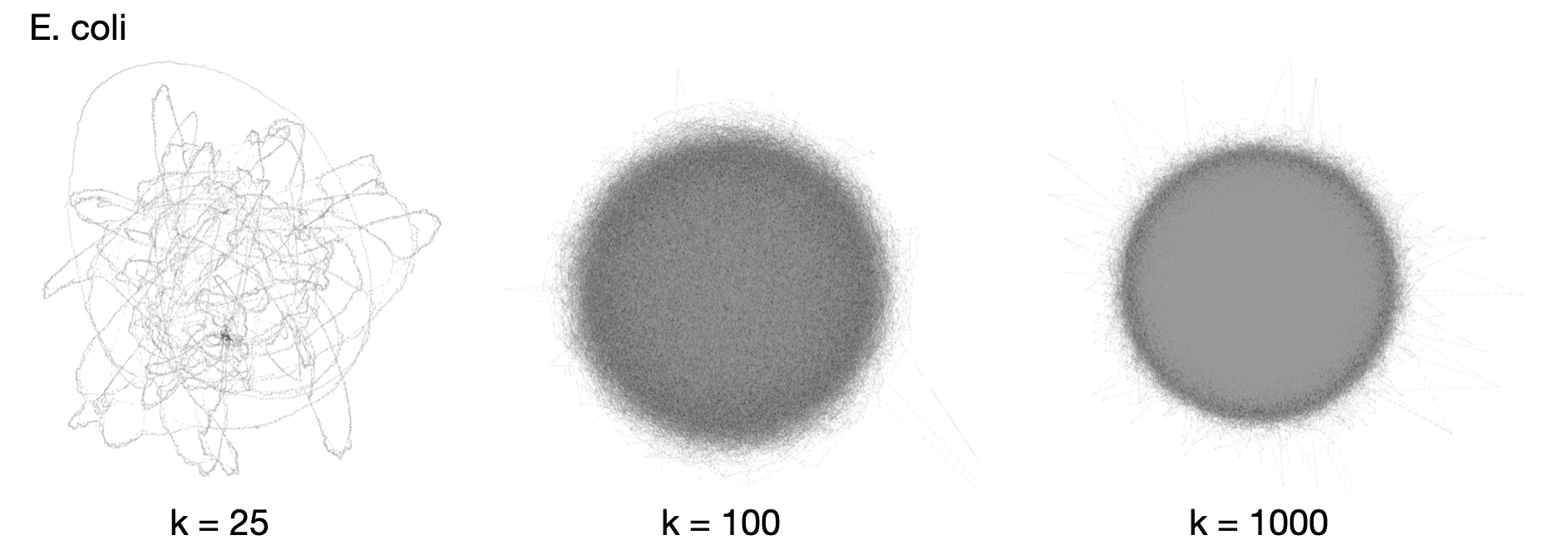
Compressed de Bruijn graphs “hairballs”: https://academic.oup.com/bioinformatics/article/30/24/3476/2422268
7.1 Set up Directories
Make sure you’re working in a screen
Make directory
- Navigate to the directory
- Link to data
7.2 Graphical Fragment Assembly (GFA) format
- Originally developed for representing genomes during assembly
- Now used for pangenomics
7.3 Bandage
Bandage: https://rrwick.github.io/Bandage/
- BLAST integration
- Can build a local BLAST database of the graph
- Can do a web BLAST search with sequences from nodes
- More details on making CSV labels: https://github.com/rrwick/Bandage/wiki/CSV-labels
Group exercise:
- Copy the following example graph from inbre to your computer using a GUI or the scp command below.
- Open Bandage and load the graph
- Spend some time exploring the graph
- If you were able to install BLAST, find CUP1 and YHR054C via BLAST. You can download them from the links or there is a fasta file on the server with both genes sequences (/home/data/pangenomics-2503/yprp/CUP1/cup1.yhr054c.fa)
- How many copies are in the graph?
- What does the structure it’s in look like?
- Take a screenshot of the region that CUP1 is in with the gene colored
7.4 BLAST the graph manually
You can also blast the graph in linux by first converting the graph to fasta format. Doublecheck that you are still in the ~/viz/ directory. Otherwise, cd into that directory.
Create a FASTA file containing the graph sequence
Build a BLAST database for the FASTA
- -in S288C.SK1.fa
- the file to build a database for
- -input_type fasta
- the input file is a FASTA
- -dbtype nucl
- the type of sequence in the input file is DNA