Chapter 10 Minigraph-Cactus

10.1 Cactus

https://github.com/ComparativeGenomicsToolkit/cactus

Reference-free whole genome graph
Constructs graph based on MSA or graph

10.2 Cactus Graphs

Cactus Graphs “naturally decompose the common substructures in a set of related genomes into a hierarchy of chains that can be visualized as two-dimensional multiple alignments and nets that can be visualized in circular genome plots”

https://www.liebertpub.com/ doi/abs/10.1089/cmb.2010.02 52

Cactus

10.3 Cactus Algorithm

Multiple sequence aligner
Originally developed for multi-species alignments
Fast because it uses a guide tree (Newick format)

https://evolution.genetics.washington.edu/phylip/newicktree.html

Now supports minigraph GFA in place of guide tree for pangenome alignments

https://github.com/lh3/minigraph

Yeast

10.4 Minigraph-Cactus

https://github.com/ComparativeGenomicsToolkit/cactus/blob/master/doc/pangenome.md https://doi.org/10.1038/s41587-023-01793-w

Minigraph-Cactus Article

Minigraph-Cactus Pipeline

10.4.1 Pipeline

Prepare the input
Build graph
Indexing, read mapping, variant calling
View with Bandage

10.4.2 Set up Directories

Make sure you’re working in a screen
Make Directory

mkdir cactus

Navigate to the Directory

cd cactus

Copy the data

cp -r /home/data/pangenomics-2503/yprp .

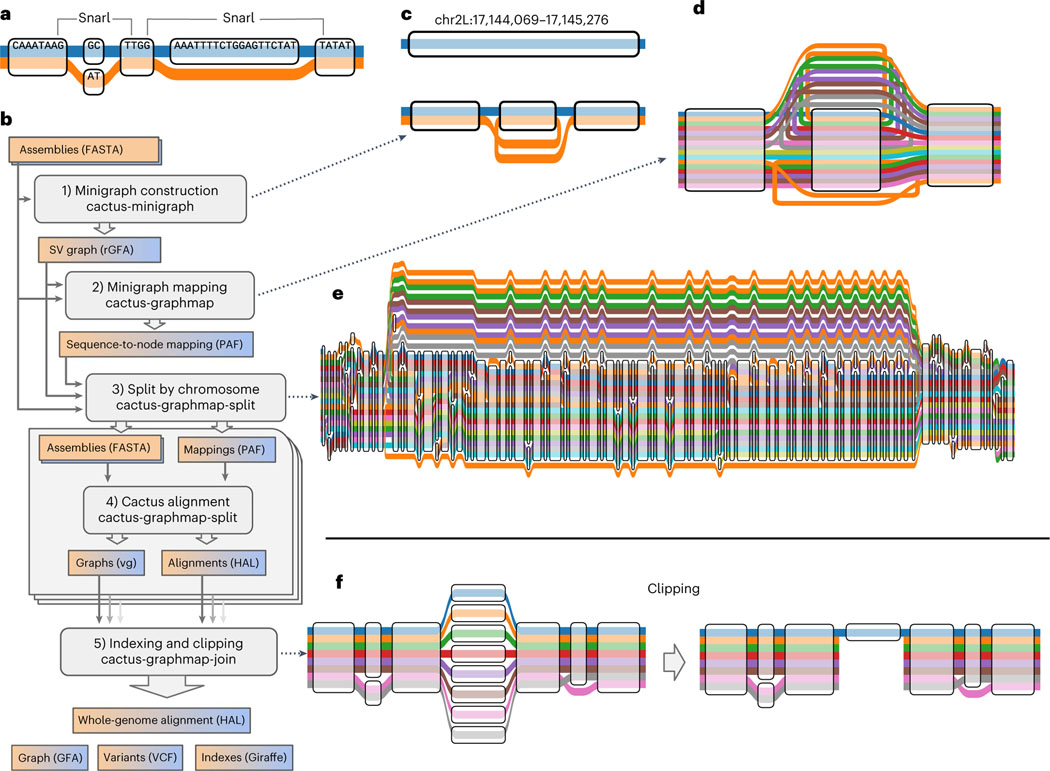
10.5 Building the Graph

10.5.1 Preparing the Input (exercise)

Cactus seqFile tells Cactus where to load sequences from

Maps sequence names to file paths
- We’re using:
```
“<strain name>\t<path to sequence>”
```

E.G.

seqFile: S288C ./yprp/assemblies/S288C.genome.fa

Call it yprp.seqfile.txt

10.5.2 Singularity

https://docs.sylabs.io/guides/latest/user-guide/

Secure containers for reproducible scientific computing
Any user can run a singularity container
Containers are portable, self-contained environments with everything a program needs to run

Singularity containers are saved in .sif files. .sif files for this workshop are stored in /home/data/pangenomics-2503/sif/.

10.5.3 Cactus

Build a graph containing all of the YPRP genomes (10min):

singularity run --no-privs /home/data/pangenomics-2503/sif/cactus.sif cactus-pangenome \
    ./js \
    ./yprp.seqfile.txt \
    --outDir yprp-cactus \
    --outName yprp-cactus \
    --reference S288C \
    --giraffe \
    --gfa \
    --gbz \
    --mgCores 10 \
    --mapCores 10 \
    --consCores 10 \
    --indexCores 10

singularity run –no-privs /home/data/pangenomics-2503/sif/cactus.sif
- run the Cactus container with singularity
cactus-pangenome
- the command to run inside the container
./js
- a job store directory where intermediate files should be stored (shouldn’t already exist)
./yprp.seqfile.txt
- the text file mapping sequence names to file paths
–outDir yprp-cactus
- a directory where output files should be stored (shouldn’t already exist)
–outName yprp-cactus
- the prefix that every output file should be given
–reference S288C
- which input sequence should be treated as the reference
–giraffe
- files for the giraffe read mapper should be generated
–gfa
- a file containing the graph in GFA format should be generated
–gbz
- a file containing the graph in GBZ format should be generated
–mgCores 10
- minigraph should use 10 CPU cores
–mapCores 10
- the mapper should use 10 CPU cores
–consCores 10
- the Cactus consolidate algorithm should use 10 CPU cores
–indexCores 10
- the indexer should use 10 cores

10.6 Read Mapping and Variant Calling

10.6.1 Reading Mapping

Map reads (10min):

vg giraffe \
    -p \
    -Z ./yprp-cactus/yprp-cactus.gbz \
    -m ./yprp-cactus/yprp-cactus.d2.min \
    -d ./yprp-cactus/yprp-cactus.d2.dist \
    -f ./yprp/reads/SK1.illumina.fastq.gz \
    -t 10 > yprp-cactus.SK1.illumina.gam

-p
- show progress
-Z ./yprp-cactus/yprp-cactus.gbz
- use the Graph Burrows-Wheeler Transform generated by Cactus
-m ./yprp-cactus/yprp-cactus.d2.min
- the minimizer index generated by Cactus
-d ./yprp-cactus/yprp-cactus.d2.dist
- the distance index generated by Cactus
-f ./yprp/reads/SK1.illumina.fastq.gz
- the reads to map
-t 10
- number of threads to use
> yprp-cactus.SK1.illumina.gam
- write the standard out (the mapped reads) into yprp-cactus.SK1.illumina.gam

Computing mapping stats (2min):

vg stats -a yprp-cactus.SK1.illumina.gam

-a
- input is an alignment (GAM) file

10.6.2 Calling Graph-Supported Variants

Compute read support for variation already in the graph (6min):

vg pack \
    -x yprp-cactus/yprp-cactus.d2.gbz \
    -g yprp-cactus.SK1.illumina.gam \
    -Q 5 \
    -s 5 \
    -o yprp-cactus.SK1.illumina.pack \
    -t 10

-x yprp-cactus/yprp-cactus.d2.gbz
- use the Graph Burrows-Wheeler Transform generated by Cactus
-Q 5
- ignore mapping and base quality < 5
-s 5
- ignore the first and last 5pb of each read
-o yprp-cactus.SK1.illumina.pack
- the output pack file
-t 10
- use 10 threads

Compute snarls in graph structure (<1min):

vg snarls yprp-cactus/yprp-cactus.d2.gbz -t 10 > yprp-cactus.snarls

yprp-cactus/yprp-cactus.d2.gbz
- use the Graph Burrows-Wheeler Transform generated by Cactus
-t 10
- use 10 threads
> yprp-cactus.snarls
- write the standard out (the snarls) into yprp-cactus.snarls

Generate a VCF from the support (<1min):

vg call \
    yprp-cactus/yprp-cactus.d2.gbz \
    -k yprp-cactus.SK1.illumina.pack \
    -r yprp-cactus.snarls \
    -t 10 > yprp-cactus.SK1.illumina.graph_calls.vcf

yprp-cactus/yprp-cactus.d2.gbz
- use the Graph Burrows-Wheeler Transform generated by Cactus
-k yprp-cactus.SK1.illumina.pack
- use the pack file we just generated
-r yprp-cactus.snarls
- use the snarls file we just generated
-t 10
- use 10 threads
> yprp-cactus.SK1.illumina.graph_calls.vcf
- write the standard out (the called variants) into yprp-cactus.SK1.illumina.graph_calls.vcf

10.6.3 Calling Novel Variants

Augmenting a single graph can take much more time than making a separate graph for each chromosome and augmenting them individually. Make a separate graph for each chromosome (1min):

vg chunk -x yprp-cactus/yprp-cactus.gbz -M -O pg -t 10

-x yprp-cactus/yprp-cactus.gbz
- use the Graph Burrows-Wheeler Transform generated by Cactus
-M
- create a chunk for each path in the graph’s connected components, i.e. each chromosome
-O pg
- the chunked graphs should be in the packed-graph format
-t 10
- use 10 threads

BUG: Change the extension of the graph chunks from .vg to .pg:

for f in *.vg; do mv -- "$f" "${f%.vg}.pg"; done

Make a directory to store all the chromosome graphs:

mkdir chunks
mv *.pg chunks/

Augment the packed-graph for chromosome 1 with the mapped reads (4min):

vg augment \
    chunks/chunk_S288C#0#S288C.chrI.pg \
    yprp-cactus.SK1.illumina.gam \
    -s \
    -m 4 \
    -q 5 \
    -Q 5 \
    -A S288C.chrI.SK1.illumina.aug.gam \
    -t 10 > S288C.chrI.SK1.illumina.aug.pg

-s
- the graph being augmented is a subgraph of the graph used to create the GAM
-m 4
- filter breakpoints with coverage less than 4
-q 5
- filter bases with quality less than 5
-Q 5
- filter mappings with quality less than 5
-A S288C.SK1.illumina.aug.gam
- output the read mappings relative to the augmented graph
-t 10
- use 10 threads
> S288C.chrI.SK1.illumina.aug.pg
- write the standard out (the augmented graph) into S288C.chrI.SK1.illumina.aug.pg

Compute read support for the augmented graph (<1min):

vg pack \
    -x S288C.chrI.SK1.illumina.aug.pg \
    -g S288C.chrI.SK1.illumina.aug.gam \
    -Q 5 \
    -s 5 \
    -o S288C.chrI.SK1.illumina.aug.pack \
    -t 10

Compute snarls in the augmented graph structure (<1min):

vg snarls S288C.chrI.SK1.illumina.aug.pg -t 10 > S288C.chrI.SK1.illumina.aug.snarls

Generate a VCF from the support (<1min)

vg call \
    S288C.chrI.SK1.illumina.aug.pg \
    -k S288C.chrI.SK1.illumina.aug.pack \
    -r S288C.chrI.SK1.illumina.aug.snarls \
    -t 10 > S288C.chrI.SK1.illumina.aug_calls.vcf

10.6.4 Exercise

Call variants on the graphs for the other chromosomes

Can you automate this with a bash script?

10.7 BLAST the graph manually

Create a FASTA file containing the graph sequence (<1min):

gfatools gfa2fa yprp-cactus/yprp-cactus.gfa.gz > yprp-cactus.fa

Build a BLAST database for the FASTA (1min):

makeblastdb -in yprp-cactus.fa -input_type fasta -dbtype nucl

Query the database for CUP1 and YHR054C (<1min):

blastn -outfmt 7 -db yprp-cactus.fa -query yprp/CUP1/cup1.yhr054c.fa > yprp-cactus.cup1.blast.tsv

10.8 Viewing with Bandage

Cactus graphs are too complex so you should only view specific subgraphs with Bandage. Here we’ll look at a subgraph of chromosome 8 that contains the CUP1 gene.

List the paths in the chromosome 8 graph (<1min):

vg paths -L -x chunks/chunk_S288C#0#S288C.chrVIII.pg

-L
- List all paths in the graph
-x chunks/chunk_S288C#0#S288C.chrVIII.pg
- The graph file to use

Compute snarls for the chromosome 8 graph (<1min):

vg snarls chunks/chunk_S288C#0#S288C.chrVIII.pg -t 10 > S288C.chrVIII.snarls

Extract the subgraph along the portion of the S288C path that contains the CUP1 gene (<1min):

vg chunk \
  -x chunks/chunk_S288C#0#S288C.chrVIII.pg \
  -S S288C.chrVIII.snarls \
  -p S288C#0#S288C.chrVIII:210000-220000 \
  -O gfa \
  -t 10 > S288C.chrVIII.210000-220000.gfa

-x chunks/chunk_S288C#0#S288C.chrVIII.pg
- the graph to chunk
-S S288C.chrVIII.snarls
- the snarls for the graph (can use -c for node distnace instead)
-p S288C#0#S288C.chrVIII:210000-220000
- the path segment to extract
-O gfa
- the output graph should be a GFA
-t 10
- use 10 threads
> S288C.chrVIII.210000-220000.gfa
- write the standard out (the graph chunk) into S288C.chrVIII.210000-220000.gfa

10.8.1 Exercise

Open with Bandage
Where’s CUP1?
Does the graph capture any CNV?
What does it look like?
Take a screenshot of the CUP1 region

10.9 Pros and Cons minigraph-cactus

Pros:

Building graphs is relatively fast
Graphs represent multiple assemblies
Handles Giraffe indexing as part of graph building

Cons:

Graphs are biased by the minigraph used to construct the graph
Graphs are hard to visualize in Bandage
Cactus pipeline is more opaque than vg construct
Only “reference” path from minigraph is embedded in graph