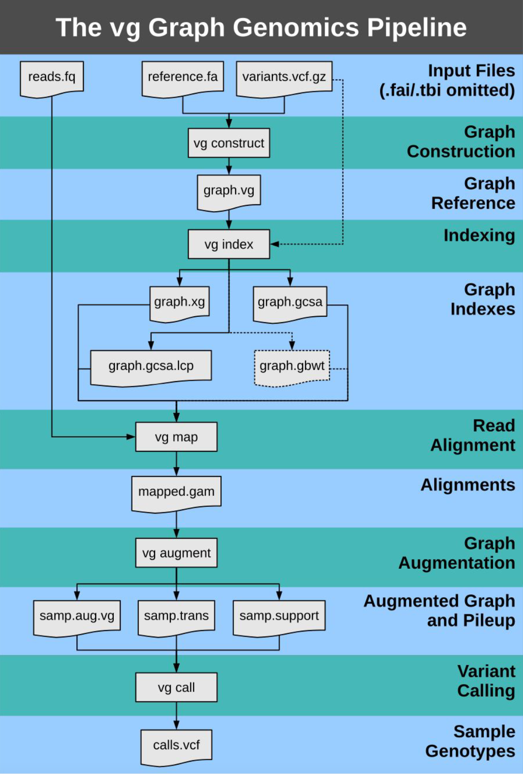
Chapter 6 VG Toolkit
6.1 Variation Graph (VG) Toolkit
- Constructs graphs
- Manipulates graphs
- Indexes graphs
- Maps sequences to graphs
- Calls variants on mapped sequences
- Visualizes graphs
Also does:
- Transcriptomic analysis
- Assembly-based pipelines
- So much more
Graphs are acyclic, but otherwise general, i.e. reference, iterative, reference-free, etc.
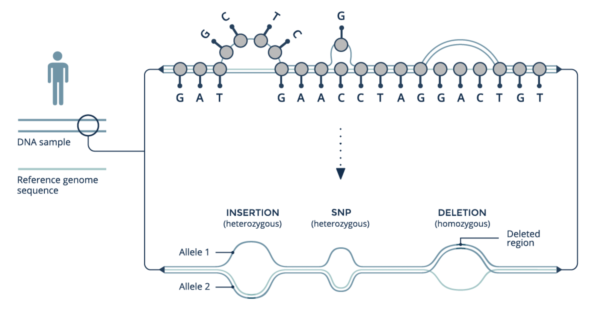
6.2 Reference Graphs
A reference genome “decorated” with variants:
6.2.2 Preparing the Input
Already done for you:
- Reference FASTA
- Description lines should only contain chromosome names
- Remove extraneous sequences, e.g. mitochondrial DNA
- VCF
- Ideally chromosome names exactly match chromosome names in reference
6.2.3 Set up directories
- Make sure you’re working in a screen
- Make directory
- Navigate to the directory
- Link to data
6.2.4 Variant Call (VCF) Format
https://en.wikipedia.org/wiki/Variant_Call_Format
- Plain text file
- Header:
- Header lines start with #
- Header lines with special keywords start with ##
- Columns
- Tab separated
- 8 mandatory columns
- CHROM, POS, ID, REF, ALT, QUAL , FILTER, INFO
- 9th column is optional
- FORMAT
- Each additional column represents a sample and has the format described in the FORMAT column
6.2.5 Variation Graph (VG) Format
https://github.com/vgteam/vg/wiki/File-Formats
- Protocol Buffer messages (protobufs) describing a graph that can store sequence in its nodes and paths
- Encoded as binary
- Code for reading/writing protobufs can be generated for many languages
- vg.proto
6.2.6 Graphical Fragment Assembly (GFA) Format
- Originally developed for representing genomes during assembly
- Now used for pangenomics
6.2.7 Yeast Data
Reference: S288C
VCF: 3 SV calling pipelines on the 11 non-reference strains
- Minimap2 and paftools call
- LAST and AsmVar
- nucmer and Assemblytics
This workshop used an updated version of the Phase 1 pipeline available here
6.2.8 Construct Graph
Construct a graph from the reference and VCF:
vg construct -r yprp/assemblies/S288C.genome.fa -v yprp/variants/S288C.vcf -S -a -f -p -t 10 > S288C.vg- -r yprp/assemblies/S288C.fa
- the reference genome
- -v yprp/variants/S288C.sv.vcf
- the VCF file containing variants (indels, structures, etc)
- -S
- include structural variants in construction of graph
- -a
- save paths for alts of variants by variant ID
- -f
- don’t chop up alternate alleles from input VCF
- -p
- show progress
- -t 10
- use 10 threads
- > S288C.vg
- write the standard out (the computed graph) into S288C.vg
Compact chains of nodes:
- -u
- unchop nodes, i.e. compact chains
6.3 Graph Indexing
6.3.2 VG Index Formats
https://github.com/vgteam/vg/wiki/File-Formats
Distance Index (.dist)
- Minimum path distance between nodes in the graph
Graph Burrows-Wheeler Transform (.gbz)
- GBWT haplotype index, augmented with a path cover of graph components without haplotypes and/or subsampled to a reasonable number of local haplotypes
- GBWTGraph that provides node sequences
Minimizer index (.min)
- Minimizers used for seed finding
Zipcodes (.zipcodes)
Zipcode annotations for finding sequence positions of minimizers
6.3.3 Indexing
VG uses the autoindex command to generate the necessary index files for various workflows.
Generate the indexes for read mapping as follows (1min):
- –workflow giraffe
- generate indexes for the “giraffe” read mapper
- -g S288C.gfa
- the
.gfafile to index
- the
- -p S2888C
- the prefix to give all generated index files
If you have a graph with haplotypes as P-lines, you must build the indexes manually. However, version 1.53.0 or later fixes this issue as long as the haplotypes are named correctly. For instance, autoindexing works for PGGB.
Graphs converted from .vg to .gfa will have haplotypes as P-lines.
vg gbwt --gbz-format -g S288C.giraffe.gbz -G S288C.gfa
vg index -j S288C.dist S288C.gfa
vg minimizer -d S288C.dist -o S288C.shortread.withzip.min S288C.giraffe.gbz- vg gbwt –gbz-format -g S288C.giraffe.gbz
- the
.gbzfile to generate
- the
- vg index -j S288C.dist
- the
.distfile to generate
- the
- vg minimizer -o S288C.shortread.withzip.min
- the
.minfile to generate
- the
6.4 Read Mapping
6.4.2 Graph Alignment/Map (GAM) Format
https://github.com/vgteam/vg/wiki/File-Formats
- Analogous to BAM, but for graphs
- Binary file describing where reads mapped to in the graph structure
- Uncompressed has one read per line
- Can be converted to JSON for manual parsing (very inefficient!)
6.4.3 Read Mapping
Map reads (9min):
vg giraffe -p -Z S288C.giraffe.gbz -m S288C.shortread.withzip.min -d S288C.dist -f yprp/reads/SK1.illumina.fastq.gz -t 10 > S288C.SK1.illumina.gam- -p
- show progress
- -Z S288C.giraffe.gbz
- the Graph Burrows-Wheeler Transform to use
- -m S288C.shortread.withzip.min
- the minimizer index to use
- -d S288C.dist
- the distance index to use
- -f yprp/reads/SK1.illumina.fastq.gz
- the reads to map
- -t 10
- number of threads to use
Computing mapping stats (<1min):
- -a
- input is an alignment (GAM) file
6.4.4 Bringing Alignments Back to Single Genomes
Map reads (1min):
- -x S288C.giraffe.gbz
- graph or xg to use
- -b
- BAM output
- -t 10
- use 10 threads
Exercise:
- Rename chromosomes in BED for use with IGV
- Copy BED to personal computer
- Spend some time looking at BED in IGV and share any interesting observations you may have?
- What’s up with CUP1?
6.5 Calling Graph Supported Variants
6.5.2 Packed-Graph Format
https://github.com/vgteam/vg/wiki/File-Formats
- A memory-efficient, dynamic graph representation
- The format isn’t actually documented…
6.5.3 Pack (pileup support) Format
https://github.com/vgteam/vg/wiki/File-Formats
- Binary file
- Computes pileup support for each read in a mapping
- The format isn’t actually documented…
6.5.4 Snarls Format
https://github.com/vgteam/vg/wiki/File-Formats
- Computes nested cyclic structure in the graph
- The format isn’t actually documented…
6.5.5 Calling Graph-Supported Variants
Convert the graph into a packed graph (<1min):
- -p
- the output should be a packed-graph
Compute read support for variation already in the graph (1min):
- -x S288C.pg
- the graph file to use (
.gfa,.gbz,.xg, etc)
- the graph file to use (
- -Q 5
- ignore mapping and base quality < 5
- -s 5
- ignore the first and last 5pb of each read
- -o S288C.SK1.illumina.pack
- the output pack file
- -t 10
- use 10 threads
Compute snarls in graph structure (<1min):
- S288C.pg
- the graph file to use (
.gfa,.gbz,.xg, etc)
- the graph file to use (
- -t 10
- use 10 threads
Generate a VCF from the support (<1min):
vg call S288C.pg -k S288C.SK1.illumina.pack -r S288C.snarls -t 10 > S288C.SK1.illumina.graph_calls.vcf- S288C.pg
- the graph file to use (
.gfa,.gbz,.xg, etc)
- the graph file to use (
6.6 Calling Novel Variants
6.6.2 Calling Variants
Augment the packed graph with the mapped reads (30min):
vg augment S288C.pg S288C.SK1.illumina.gam -m 4 -q 5 -Q 5 -A S288C.SK1.illumina.aug.gam -t 10 > S288C.SK1.illumina.aug.pg- -m 4
- filter breakpoints with coverage less than 4
- -q 5
- filter bases with quality less than 5
- -Q 5
- filter mappings with quality less than 5
- -A S288C.SK1.illumina.aug.gam
- output the read mappings relative to the augmented graph
- -t 10
- use 10 threads
- > S288C.SK1.illumina.aug.pg
- write the standard out (the augmented graph) into S288C.SK1.illumina.aug.pg
Compute read support for the augmented graph (2min):
vg pack -x S288C.SK1.illumina.aug.pg -g S288C.SK1.illumina.aug.gam -Q 5 -s 5 -o S288C.SK1.illumina.aug.pack -t 10Compute snarls in the augmented graph structure (<1min):
Generate a VCF from the support (3min)
6.8 Calling Variants Already in the Graph
Output variants used to construct graph (<1min):
- -P S288C
- report variants relative to paths with names that start with S288C
S288C.deconstruct.vcf might not be identical to S288C.vcf because VG takes liberties with variants when constructing the graph.
6.9 Pros and Cons Reference Graphs
Pros:
- Graphs are relatively small
- Easy to inspect visually
- Good for low-quality / fragmented assemblies
- Shorter run-times
Cons:
- Variation represented is determined by VCF pipeline
- Only describes variation relative to the reference
- Suboptimal mappings
- Suboptimal population structure
6.10 Additional vg Commands that are Useful
6.10.1 vg combine
Combines two or more graphs into one.
- Use to construct graph in parts (e.g. individual chromosomes) and then combine
- Use to combine graphs of related species
6.10.2 Modifying and Simplifying Graphs
vg chunk - Splits graphs or alignments into smaller chunks.
vg mod - Used to modify graphs.
- We’ve already used vg mod -u to “unchop” nodes.
vg simplifying - Simplifies a graph.
vg find - Used to identify subgraphs based on various metrics and parameters.
- e.g. anchored by a region on a specific chromosome.
Use –help with any command to learn how to use it.
6.11 Drawing Graphs
vg view - Outputs graphs and other structures for drawing.
- We’ve already used vg view -g to convert from vg to gfa for viewing in Bandage.
- Can also output dot (among other files types) which is a more general graph drawing format (compatible with Graphviz).
vg viz - Basic graph drawing (documentation).
- Recommend only using on small (sub)graphs.
- Use in conjunction with chunk, mod, and/or find to draw an interesting subgraph.
- You can include mapped reads in the visualization!