Chapter 9 Minigraph
9.2 Minigraph Overview
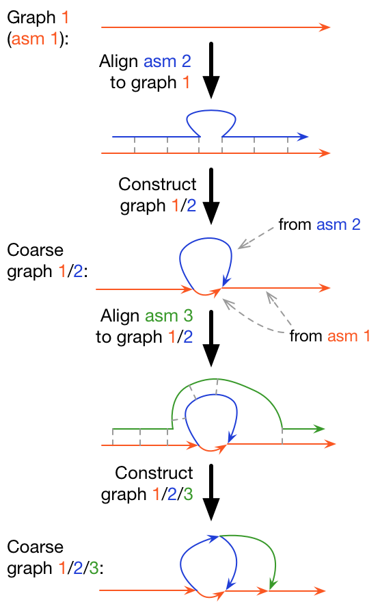
Maps diverged sequences and adds them into the graph iteratively. It is not reference-free nor does it aim to find every single variant, but it does well in finding structural variants.
Here we will build and analyze a minigraph pangenome graph then use it to create a reference-free pangenome graph in cactus.
9.3 Minimizers and Minimap2
Minigraph is built off of ideas and code from Minimap2.
Minimizers
From the minimap2 usage: “A minimizer is the smallest k-mer in a window of w consecutive k-mers.”
Essentially a minimizer tags a sequence window with the kmer that is first alphabetically.
A nice tutorial:
+ https://homolog.us/blogs/bioinfo/2017/10/25/intro-minimizer/
Minimap2
Minimap2 is a fast sequence aligner. It can align short or long reads or assemblies against a reference using the seed-chain-align approach that many aligners employ. It finds exact matches (anchors) between query minimizers (seeds) and indexed reference minimizers. It links colinear anchors together (chains). For nt-level alignment it fills in regions between anchors within chains and between chains (align).
https://github.com/lh3/minimap2
https://academic.oup.com/bioinformatics/article/34/18/3094/4994778
9.4 Pipeline
- Prepare the input
- Build graphs
- Build a single genome graph and incrementally add more sequences
- Or build a graph for all sequences at once
- View with Bandage
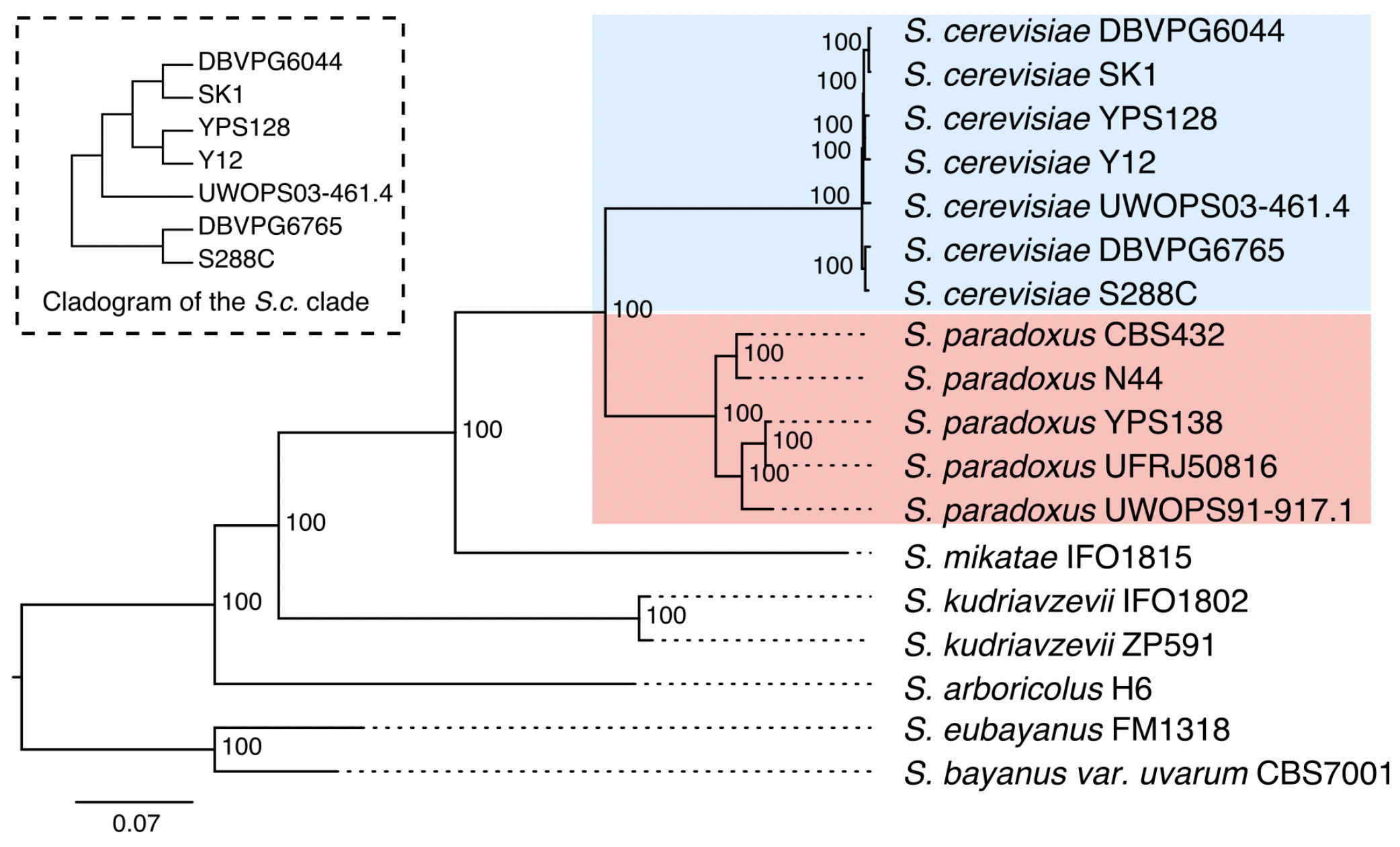
9.5 Yeast Assemblies
12 Mb
16 chromosomes
Yeast Population Reference Panel (YPRP) https://yjx1217.github.io/Yeast_PacBio_2016/data/
12 Yeast PacBio Assemblies (Chromosome level)
- ~100-200x PacBio sequencing reads
- HGAP + Quiver polishing
- ~200-500x Illumina (Pilon correction)
- Manual curation
- Annotation
Make sure your chromosome names are unique across all samples and that they contain the sample name. We’re using <strain name>.<chromosome> (>S288C.chrVIII)
9.6 Prepare the Input
Make sure you’re working in a screen
Make Directory
- Navigate to the Directory
- Link to data
9.7 Graphical Fragment Assembly (GFA) format
Tab-delimited text
Lines start with one of the following types:
| Type | Description | Explanation |
|---|---|---|
| H | Header | |
| S | Segment | A continuous sequence or subsequence |
| L | Link | Segment overlaps (basepairs & orientations) |
| J | Jump | Jumps link sequences across gaps |
| C | Containment | Segment contained in another segment |
| P | Path | An ordered & oriented list of linked segments |
| W | Walk | An ordered & oriented list of segments w/o overlaps |
| # | Comment |
Optional Fields TAG:TYPE:VALUE
http://gfa-spec.github.io/GFA-spec/GFA1.html
Let’s go to the specification to look at optional fields and an example:
http://gfa-spec.github.io/GFA-spec/GFA1.html
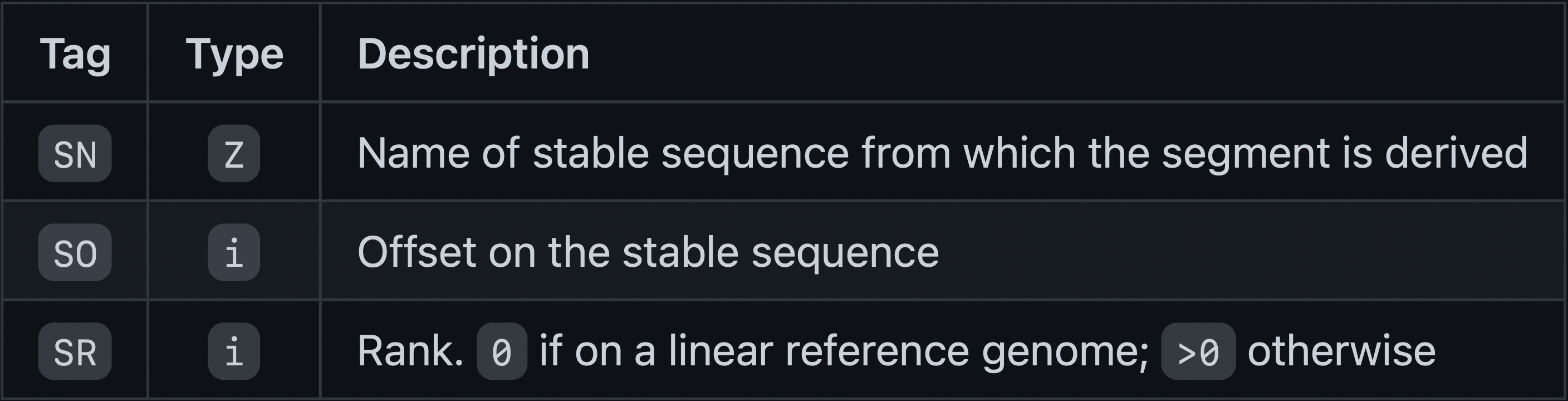
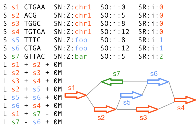
9.8 reference Graphical Fragment Assembly (rGFA)
https://github.com/lh3/gfatools/blob/master/doc/rGFA.md
- Strict subset of GFA
- Tags that trace origin
- Stable coordinates
9.9 Build rGFA Graphs
- The first sequence in the graph is used as a “reference”:
- -xggs
- build a graph using a simple (ggs) algorithm
- -t 20
- use 20 threads (default is 4)
- -c
- perform base alignment; RECOMMENDED
“Please add option -c for graph generation as it generally improves the quality of graphs.”
- Incrementally add strains to graph:
minigraph -cxggs ref.minigraph.gfa strain_1.fa > strain_1.minigraph.gfa

minigraph -cxggs strain_1.minigraph.gfa strain_2.fa > strain_2.minigrpah.gfa
...

minigraph -cxggs string_N-1.gfa strain_N.fa > yprp.minigraph.gfa- Or build a graph for all strains at once:
9.10 Reference Graph
Let’s create a graph for the reference (S288C) and answer the following questions. This is a small dataset so we’ll use the default threads (4).
- Make the reference graph
- How many lines in the gfa file?
- What type of lines are they?
9.11 YPRP Graphs
- Add in the rest of the lines
- we’ll do this alphabetically
- capture the stderr
minigraph -xggs -c ref.minigraph.gfa $(ls *.fa | grep -v S288C) > yprp.minigraph.gfa 2>yprp.minigraph.errNote: We can simply use the reference fasta instead of a gfa
minigraph -xggs -c S288C.genome.fa $(ls *fa | grep -v S288C) > yprp.minigraph.gfa 2>yprp.minigraph.errTry to answer the following questions:
- How many lines are in the gfa file?
- What type of lines are they?
- How many yeast assemblies have inversions compared to S288C (hint: look in the stderr)?
Click for Answer
[M::mg_ggsimple_cigar::11.337*2.72] inserted 1791 events, including 0 inversions
[M::mg_ggsimple_cigar::17.749*2.88] inserted 336 events, including 0 inversions
[M::mg_ggsimple_cigar::22.268*2.92] inserted 176 events, including 0 inversions
[M::mg_ggsimple_cigar::27.169*2.95] inserted 451 events, including 1 inversions
[M::mg_ggsimple_cigar::35.508*2.90] inserted 56 events, including 2 inversions
[M::mg_ggsimple_cigar::49.950*3.02] inserted 728 events, including 0 inversions
[M::mg_ggsimple_cigar::53.680*2.96] inserted 208 events, including 5 inversions
[M::mg_ggsimple_cigar::62.465*3.01] inserted 679 events, including 0 inversions
[M::mg_ggsimple_cigar::72.274*3.04] inserted 134 events, including 1 inversions
[M::mg_ggsimple_cigar::79.327*3.04] inserted 117 events, including 0 inversions
[M::mg_ggsimple_cigar::82.656*3.06] inserted 258 events, including 1 inversions
10 inversions total (in 5 samples)
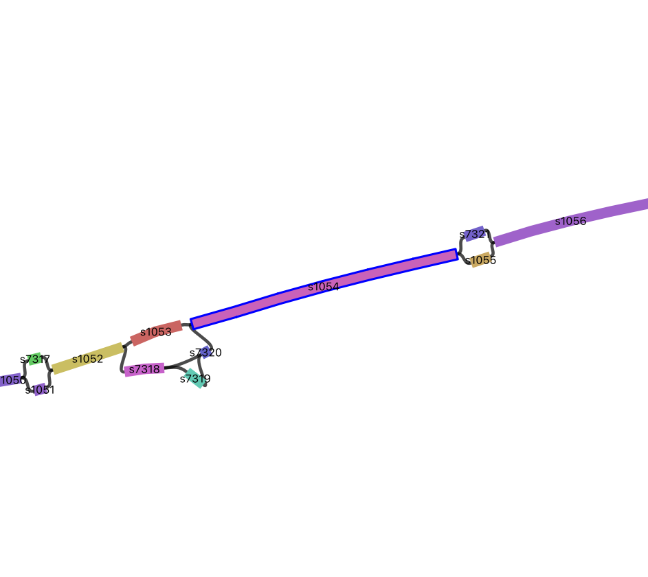
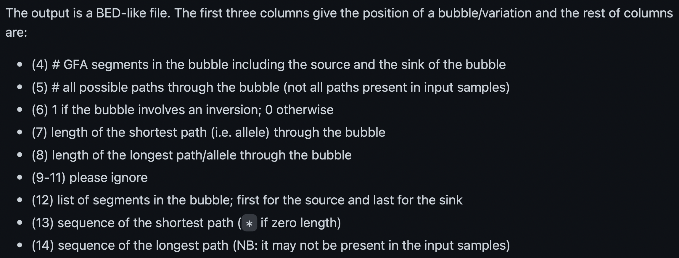
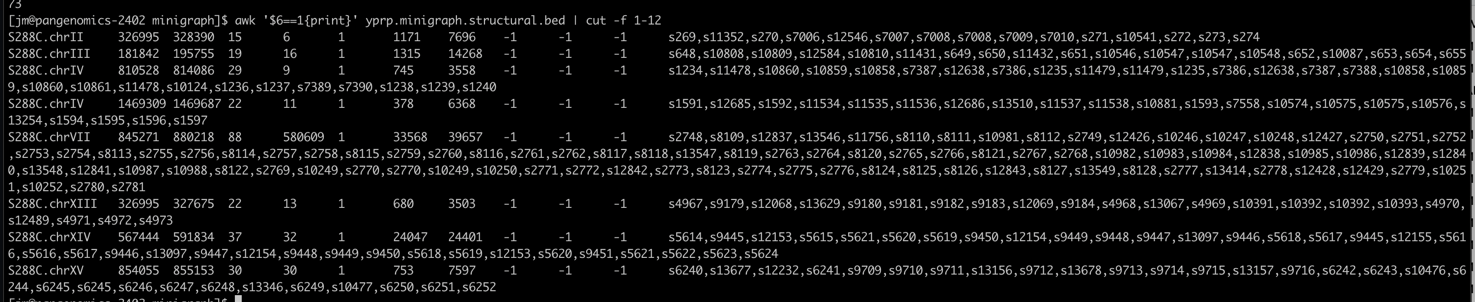
9.12 Structures in the graph
Insertions and Diverged Regions
Search for segment s1054 then zoom out a little so you can see the segments around it.
Trace the S288C path (hint: the S288C segments are numbered sequentially with the lower segment numbers).
Identify insertions and regions that have diverged.
Group Exercise
- Find a simple and a complex region
- Discuss it in your group
- Share it with everyone
- Keep track of the segments
Inversions
Here are some examples of inversions.
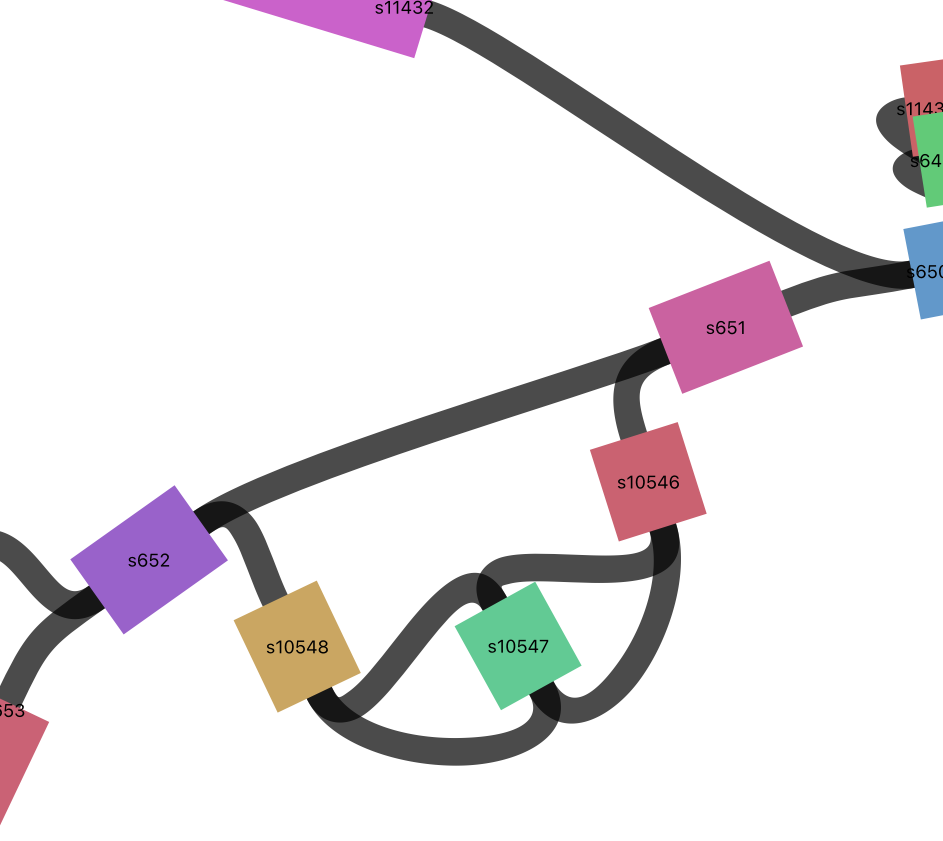
Let’s find them in bandage.
s7008
s10547
Click on the node and surrounding nodes to see how long they are.
Click on the links (black) to see the direction that paths can travel.
Click on the inverted node Choose “Color by continguity” under “Graph Display” then click on “Determine contiguity” to see which nodes the inverted node connects to.
Do a web-blast in Bandage to see what they might code for (click on the node then choose from the Output menu: Web Blast Selected Nodes). Also blast the adjacent segments to get some context.
blastn will do a nucleotide to nucleotide alignment (default) or you can choose blastx to blast it against a protein database (if it isn’t coding there won’t be any hits).
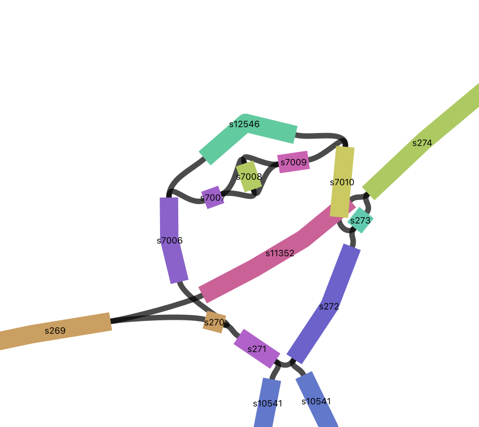
Inversions in the GFA
I found the inversions by searching the graph GFA file for pairs of segments that have two links between them. Give it a try.
  2 s10391  s10392\
  2 s10392  s10393\
  2 s10546  s10547\
  2 s10547  s10548\
  2 s10574  s10575\
  2 s10575  s10576\
  2 s10704  s10518\
  2 s6244   s6245\
  2 s6245   s6246\
  2 s7007   s7008\
2 s7008 s7009- Pull out s7008, its adjacent segments and the links connecting them
-l STR/@FILE. segment list to subset [ ]
-r INT. subset radius (effective with -l) [0]
Showing just the links here:
L s7007 + s7008 + 0M SR:i:1 L1:i:33 L2:i:381
L s7007 + s7008 - 0M SR:i:4 L1:i:33 L2:i:381
L s7008 + s7009 + 0M SR:i:1 L1:i:381 L2:i:305
L s7008 - s7009 + 0M SR:i:4 L1:i:381 L2:i:305
Now do the same for s10547
Try extending the surrounding region by increasing the -r parameter
Note: you can pull out subgraphs like these and load them into Bandage. This is helpful if the graphs are really large and slow to load.
9.13 Questions
- What is the longest segment in the graph? [Hint: Parse out the number from the 4th field of the segment line]
- What is the shortest segment in the graph?
- What cigar strings exist for the overlaps in the links? [Hint: Field 6 of the link line]
- How many segments are attributed to each genome? [Hint: Parse out field 5 of the segment line]
Click for Answer
- What is the longest segment in the graph?
- What is the shortest segment in the graph?
- What cigar strings exist for the overlaps in the links? [Hint: Field 6 of the link line]
- How many segments are attributed to each genome?
Note: There are lots of ways to do this.
9.14 Graph to Fasta
We can convert the gfa graph file to a fasta file the represents the sequence of the pangenome.
Fasta format:
>header
ACGCGCTAGCGCGAC
ACGGCGTAGGGGCAG
ACGGCT
9.15 GAF format (read alignments)
“The only visual difference between GAF and PAF is that the 6th column in GAF may encode a graph path like >MT_human:0-4001<MT_orang:3426-3927 instead of a contig/chromosome name.”
https://github.com/lh3/minigraph
Let’s look at PAF format https://lh3.github.io/minimap2/minimap2.html
9.16 Read Mapping
Align reads from SK1 to the minigraph
21,906,518 paired Illumina reads
Read length = 151 nts
minigraph -x sr yprp.minigraph.gfa /home/data/pangenomics-2402/yprp/reads/SK1.illumina.fastq.gz -t 20 > SK1.mapped.gaf-x sr map short reads (sr)
9.17 Read Mapping Stats
In theory, we could convert from GAF to GAM using vg convert then calculate stats with vg stats but the conversions doesn’t work.
Count the number of primary alignments
17298728 primary alignments
Calculate the percent of reads that had alignments
17298728/21906518 = 78.97% of reads aligned
9.18 Structural Variant Calling
Call structural variants with gfatools (doesn’t work with VG graphs last time I checked):
9.19 CUP1
Visualize the CUP1 region
10 working copies + 1 pseudogene in S288C

- Find the region in the graph based on its S288C coordinates
S288C.chrVIII:213045-233214
- Create a .csv to bring in the segment names
Note that you need a header
- Load the graph and the .csv file into Bandage
The picture below compares only S288C and SK1.
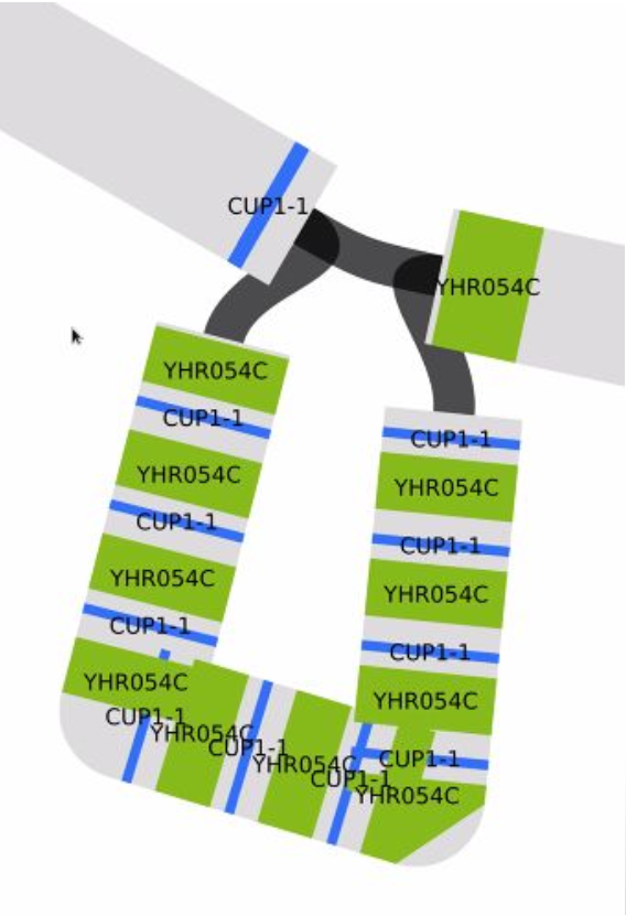
Blast the two gene sequences to their positions. CUP1 is the smaller one. Gene sequences are in: /home/data/pangenomics-2402/yprp/CUP1/cup1.yhr054c.fa
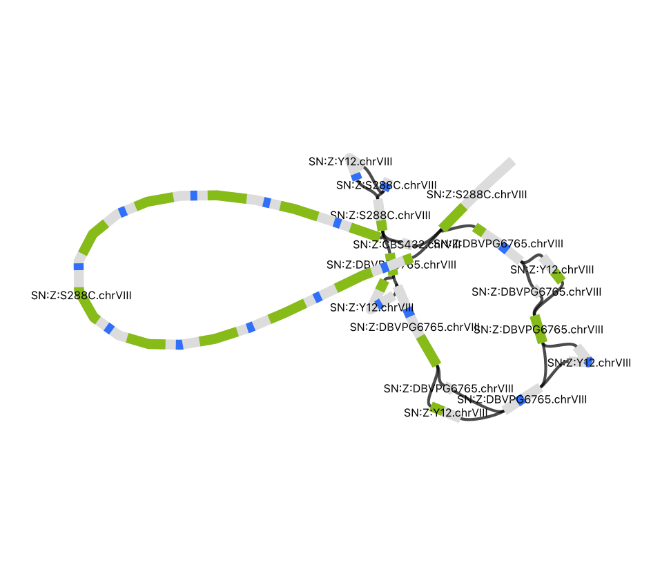
CUP1 Paths in Y12
Let’s find the Y12 paths through the graph for all bubbles in the CUP1 graph file. We will align the Y12 genome fasta to the CUP1 graph.
S288C.chrVIII 213241 213241 >s3003 >s3004 >s13286:1157:+:Y12.chrVIII:206412:207603 S288C.chrVIII 213912 233912 >s3004 >s3006 >s10622>s13287>s10623>s13288>s10625>s13289>s10626>s13290>s10628:10263:+:Y12.chrVIII:208238:218516
alignment path through the bubble:path length:mapping strand:the contig name:approximate contig start:approximate contig end
9.20 Minigraph Pros and Cons
Pros
Captures length variation
Efficient
Easy to add new genomes
Cons
Sample input order dependency
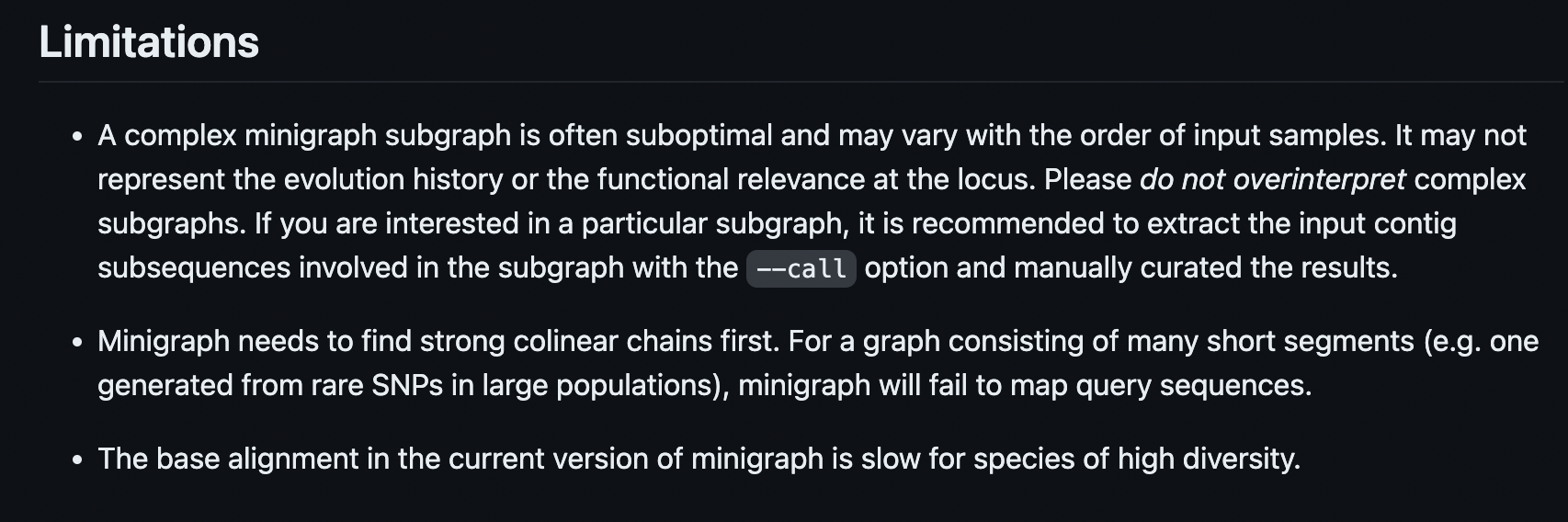
Needs collinear chains so it doesn’t work well with many short segments such as rare SNPs.
https://github.com/lh3/minigraph#limitations
9.21 Minigraph Exercises
Start with another reference
- What reference did you choose?
- What order are the other samples in?
- How does the graph compare?
- How does read mapping compare?
- How do structural variant calls compare?
- How does the cup1 region compare?
- Any other interesting differences?
Another Yeast Dataset
A subset of yeast genomes from: https://www.nature.com/articles/s41586-018-0030-5.pdf We will use 127 of these genomes.
Data are in: /home/data/pangenomics-2402/1011yeast/assemblies/A*fa.gz
Note that 1011genomes.fasta.gz in the same directory contains all of the assemblies. You can use that for cuttlefish but if you use it for minigraph it will treat it as one assembly and try to put it in the graph all at once. So, use the individual assemblies.
- How many sequences in each assembly? Min? Max?
- Make and characterize a minigraph
- Choose 13 lines to match the number of genomes we ran earlier
- Try all 127 assemblies
- How do these graphs compare to our previous yeast graph?
- Pick a region from one of the graphs and make and characterize a subgraph. Visualize it in Bandage.
Human GFA
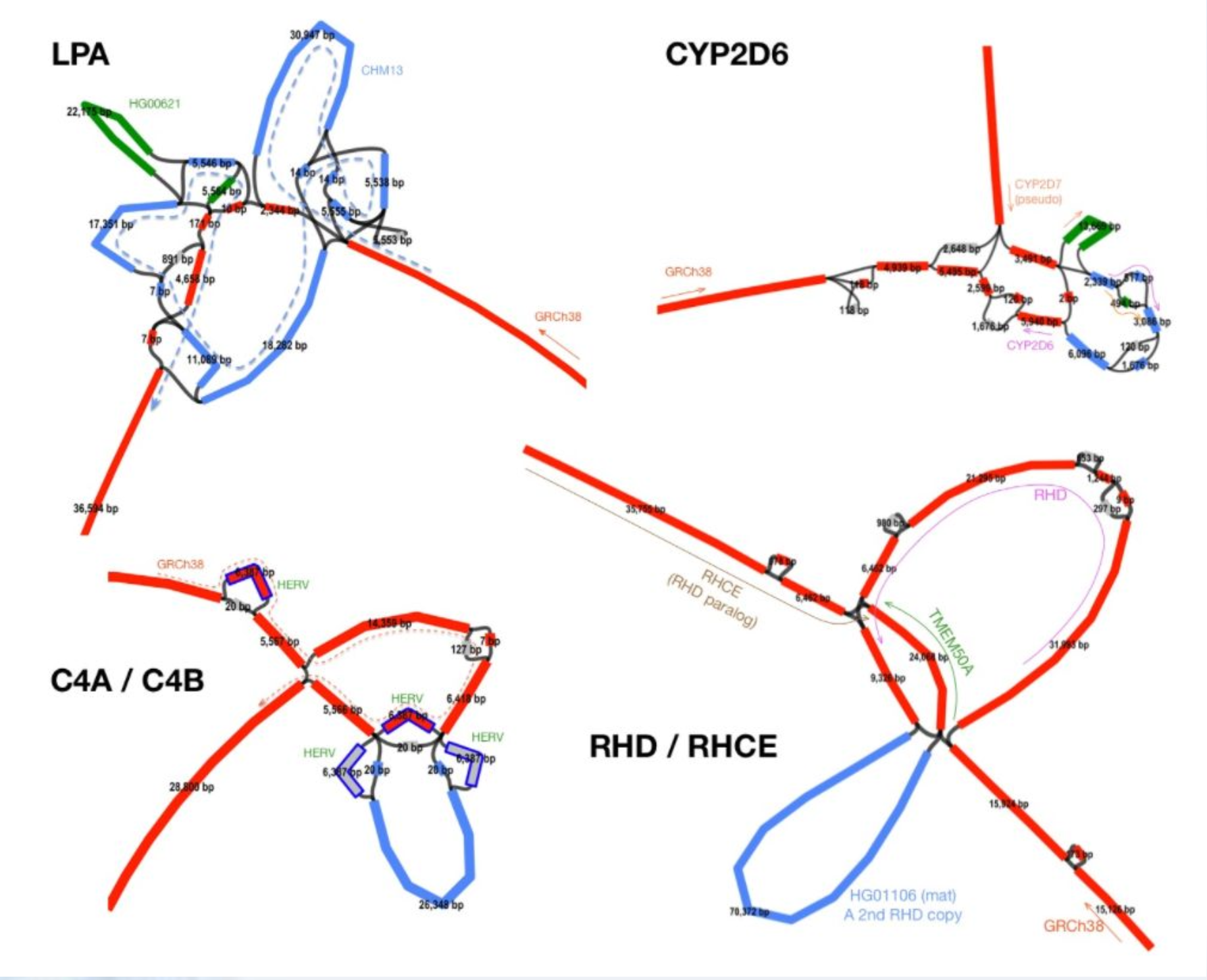
lipoprotein(a) - LPA
The LPA gene is associated with coronary heart disease. It is highly variable and includes an intragenic copy number variation where one of the domains (KIV-2) can be present in 1 to 40+ copies, separated by introns.
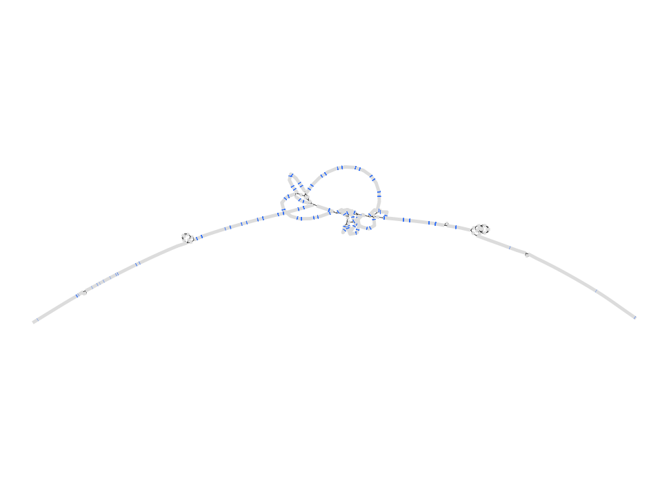
This is how it looks in an older minigraph human pangenome with CHM13 as the base.
 http://lh3.github.io/2021/01/11/minigraph-as-a-multi-assembly-sv-caller
There are a variable number of small exons in the gene.
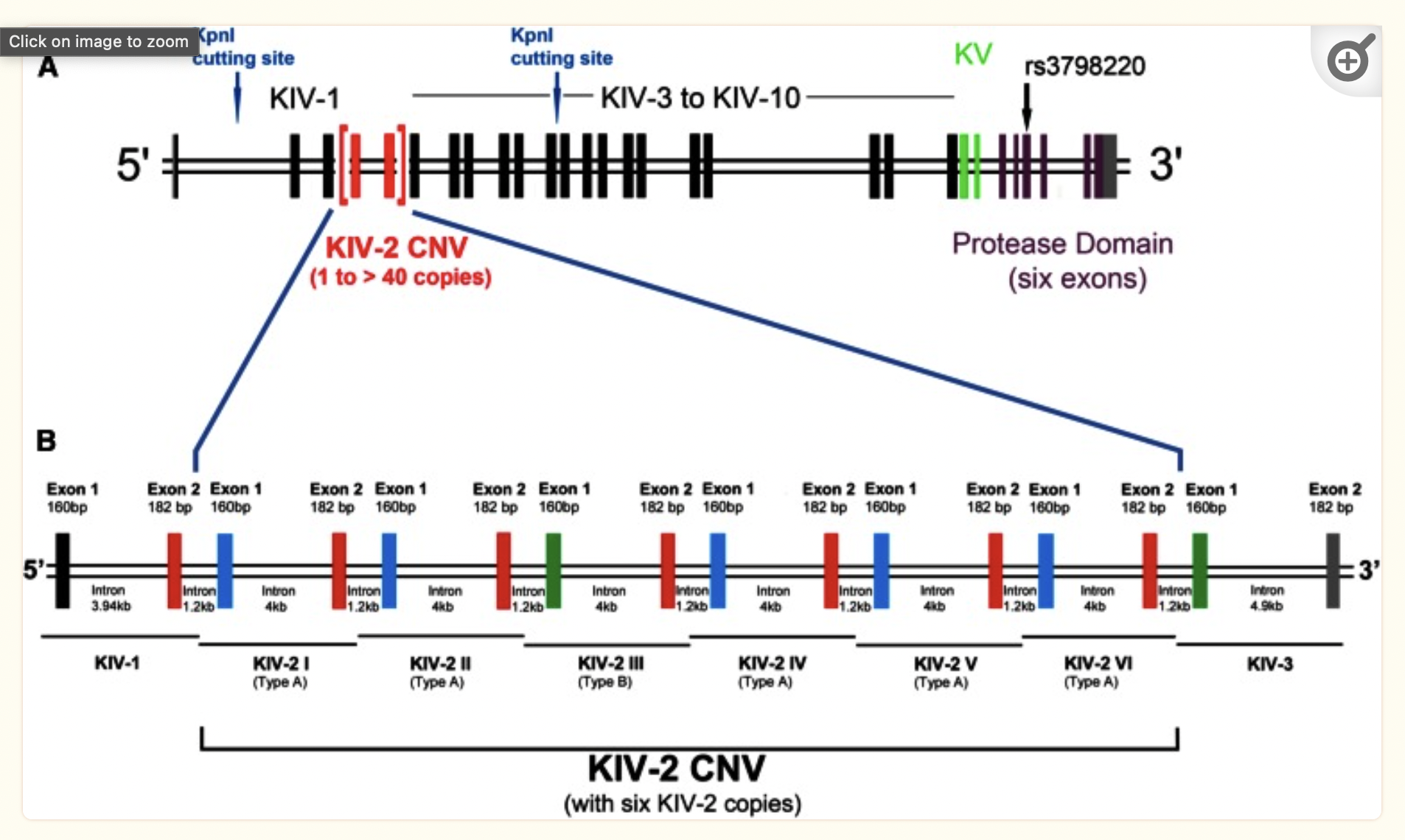
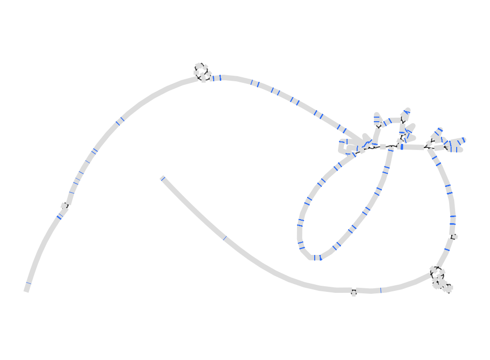
See if you can pull out and visualize the LPA region pictured below from minigraph draft human pangenome reference that uses the GRCh38 human reference genome as its base genome (https://www.nature.com/articles/s41586-023-05896-x). BLAST the LPA gene against the graph in Bandage.
Note: The GFA file is huge so don’t try to download it and upload it into bandage. Pull out a subgraph and work with that.
The GFA file is here: /home/data/pangenomics-2402/human/graphs/hprc-v1.0-minigraph-grch38.gfa.gz (no need to unzip it). The LPA gene sequence is in /home/data/pangenomics-2402/human/genes/.
The LPA coordinates for GRCh38 are chr6:160531482-160664275
Note: The base genome is labelled as just chr6 whereas additional genomes have the sample name prepended before the chr.
There is also a graph with the CMH13 reference as the base genome in the same graph folder. It’s LPA coordinates are chr6:161783172-162011762. See how that looks in Bandage.
Click for Answer
GRCh38
gfatools view -R chr6:160531482-160664275 /home/data/pangenomics-2402/human/graphs/hprc-v1.0-minigraph-grch38.gfa.gz > human.lpa.gfa
CHM13
gfatools view -R chr6:161783172-162011762 /home/data/pangenomics-2402/human/graphs/hprc-v1.0-minigraph-chm13.gfa.gz > human.lpa.chm13.gfa
Convert to VG and call variants
Convert minigraph to vg (<1min):
-g input GFA graph -p output in PackedGraph format [default]
Note that for this and other vg commands you can use -t to increase the number of threads. Our dataset is small so we won’t bother.
See https://github.com/vgteam/vg/wiki/File-Formats for more info on the PackedGraph format. Note that it is a binary format so if you want to look at it use “vg view”.
Make vertices small enough (<=1024bp) for indexing (<1min):
-X max node size
NOTE: Converting to VG isn’t required if not calling variants, i.e. you can index and map directly on GFA.
- Use vg to index the VG graph (2min)
- Use vg to map SK1 reads to minigraph GFA (17min)
- Use vg to call variants on read mapping GAM
- pack (20min)
- call (<1min)
- don’t do augment; run-time too long!