3 R basics
In this module, we will review many common and useful R commands.
If you have not already done so, login to the NCGR server and use mkdir to create a subdirectory called ‘single-cell-workshop’ in your home directory.
$ mkdir single-cell-workshopTo launch R from the Linux command line, type
$ RYou should see a welcoming message like
R version 4.5.1 (2025-06-13) -- "Great Square Root"
Copyright (C) 2025 The R Foundation for Statistical Computing
Platform: x86_64-redhat-linux-gnu

R is free software and comes with ABSOLUTELY NO WARRANTY.
You are welcome to redistribute it under certain conditions.
Type 'license()' or 'licence()' for distribution details.

  Natural language support but running in an English locale

R is a collaborative project with many contributors.
Type 'contributors()' for more information and
'citation()' on how to cite R or R packages in publications.

Type 'demo()' for some demos, 'help()' for on-line help, or
'help.start()' for an HTML browser interface to help.
Type 'q()' to quit R.

>
The > at the bottom is the R command prompt, analogous to $ in Linux.
3.1 Basic commands
Before we begin, note that R commands have a different syntax than those in Linux. While the arguments of a Linux command line follow the command itself and are separated by spaces, like
$ cd ~/single-cell-workshopR commands are functions that take arguments in parentheses, separated by commas. The R analog of Linux’s cd is setwd(), and both require one argument, the name of the directory you wish to enter.
> setwd("~/single-cell-workshop")3.1.2 Help
You can get information about any R function by typing ? plus its name. For example, to see what the getwd() function does,
?getwdTo exit help mode, type “q”.
rnorm(). What does it do? What are its arguments (input parameters)?
Click for answer
?rnormrnorm(n, mean = 0, sd = 1) returns a vector of n normally distributed random numbers, centered at mean and with standard deviation sd. Its arguments are n, mean, and sd. Only n is required, mean and sd are optional and have default values 0 and 1 respectively.
3.1.3 Packages
R is useful for much more than statistical programming, and you may enhance its basic functionality by installing special-purpose libraries (packages) such as ggplot2.
All packages used in this workshop are already installed on the NCGR server. To install them on your own computer, you would use install.packages().
# install.packages("ggplot2")RStudio also lets you install packages through its Tools menu.
3.2 Calculations and variable assignment
The simplest R operation is to compute and print out a value. (You may think of R as a giant command-line calculator.)
6*7## [1] 42sqrt(64)## [1] 8substring("Bioinformatics", 4, 7)## [1] "info"Either the <- or = operator assigns a value (the right-hand side) to a variable (the left-hand side).
x <- 4*9
x
## [1] 36y = sqrt(x)
y## [1] 6z <- x + y
z## [1] 423.3 Atomic data types
Basic R data types include
numeric for numbers in general,
integer for whole numbers,
character for text strings,
logical for Boolean (TRUE/FALSE) values,
and factor for categorical values. Factors are used to represent each category as an integer with a character label, in order to conserve memory by not repeating the same label multiple times.
To determine the type of a variable, use class().
3.3.1 Conversion between types
x <- "3.14159"
class(x)
## [1] "character"y <- as.numeric(x)
y## [1] 3.14159class(y)## [1] "numeric"z <- as.integer(x)
z## [1] 3class(z)## [1] "integer"In the last case, as.integer() rounded z down to 3.
3.3.2 Error quantities
An error occurs if you try to convert a value to an incompatible type.
s <- "Bioinformatics"
as.numeric(s)
## Warning: NAs introduced by coercion## [1] NAas.logical(s)## [1] NAThese examples produce the error value NA, which implies an undefined quantity. Another error value is NULL which represents a nonexistent quantity. (We will see an example below.)
3.4 More complex data types
3.4.1 Vector
A vector is a one-dimensional sequence of data, all of the same type. There are several ways to create one:
# Implicit increment by 1
1:5
## [1] 1 2 3 4 5# Implicit decrement by 1
10:6## [1] 10 9 8 7 6# Explicit step size
seq(0, 1, by = 0.1)## [1] 0.0 0.1 0.2 0.3 0.4 0.5 0.6 0.7 0.8 0.9 1.0# Explicit number of terms
seq(4, 5, length.out = 8 + 1)## [1] 4.000 4.125 4.250 4.375 4.500 4.625 4.750 4.875 5.000# Repeat the sequence n times
rep(1:3, times = 4)## [1] 1 2 3 1 2 3 1 2 3 1 2 3# Repeat each term of the sequence n times
rep(1:3, each = 4)## [1] 1 1 1 1 2 2 2 2 3 3 3 3# Specify your own vector using c()
british_cheeses <- c("Caerphilly", "Cheddar", "Cheshire", "Dorset Blue Vinney", "Double Gloucester", "Lancashire", "Red Leicester", "Red Windsor", "Sage Derby", "Stilton", "Wensleydale", "White Stilton")
british_cheeses## [1] "Caerphilly" "Cheddar" "Cheshire"
## [4] "Dorset Blue Vinney" "Double Gloucester" "Lancashire"
## [7] "Red Leicester" "Red Windsor" "Sage Derby"
## [10] "Stilton" "Wensleydale" "White Stilton"To take a subset of a vector, use brackets: vector[i]
# 7th element
british_cheeses[7]## [1] "Red Leicester"# 1st through 5th elements
british_cheeses[1:5]## [1] "Caerphilly" "Cheddar" "Cheshire"
## [4] "Dorset Blue Vinney" "Double Gloucester"# 2nd, 3rd, and 5th elements
british_cheeses[c(2, 3, 5)]## [1] "Cheddar" "Cheshire" "Double Gloucester"# All except the first 6 elements: negative indices
british_cheeses[-(1:6)]## [1] "Red Leicester" "Red Windsor" "Sage Derby" "Stilton"
## [5] "Wensleydale" "White Stilton"british_cheeses.
Click for answer
british_cheeses[c(2, 4, 6, 8, 10, 12)]or
british_cheeses[seq(2, length(british_cheeses), by = 2)]## [1] "Cheddar" "Dorset Blue Vinney" "Lancashire"
## [4] "Red Windsor" "Stilton" "White Stilton"The brackets may include a condition instead of an index set, for example this returns all cheeses beginning with ‘C’.
british_cheeses[startsWith(british_cheeses, "C")]## [1] "Caerphilly" "Cheddar" "Cheshire"To inspect the beginning or end of a vector, you may use the head() and tail() functions. These take an optional second argument, the number of items to display (the default is 6).
head(british_cheeses)## [1] "Caerphilly" "Cheddar" "Cheshire"
## [4] "Dorset Blue Vinney" "Double Gloucester" "Lancashire"tail(british_cheeses, 2)## [1] "Wensleydale" "White Stilton"3.4.2 Matrix
A matrix is a two-dimensional grid of data, all of the same type. You can create them from a vector plus the number of rows and/or columns, as long as nrow*ncol is a multiple of the input vector length (or you use a single value instead of a vector).
The default behavior is to fill in each column (top to bottom) before starting the next, but you may specify byrow = TRUE to fill in each row (left to right) instead, which is often more intuitive.
my_matrix_by_column <- matrix(1:6, nrow = 2, ncol = 3)
my_matrix_by_column## [,1] [,2] [,3]
## [1,] 1 3 5
## [2,] 2 4 6my_matrix <- matrix(1:6, nrow = 2, ncol = 3, byrow = TRUE)
my_matrix## [,1] [,2] [,3]
## [1,] 1 2 3
## [2,] 4 5 6To subset a matrix, use brackets:
# Element (i, j)
my_matrix[1, 2]## [1] 2# ith row: mx[i, ]
my_matrix[2, ]## [1] 4 5 6# jth column: mx[, j]
my_matrix[, 3]## [1] 3 6# Submatrix
my_matrix[1:2, c(1, 3)]## [,1] [,2]
## [1,] 1 3
## [2,] 4 63.4.3 Data frame
A data frame is a two-dimensional table in which each row represents a measurement or observation, and each column represents a different measured or observed variable. All data in each column are therefore the same type (in other words, each column is a vector), but different columns may have different types.
Here we create a data frame with the results of a cheese tasting where 100 guests (labeled 1-100) sampled 3 of the British cheeses (Cheddar, Lancashire, and Stilton) and assigned each one a flavor score and a texture score (normally distributed around the mean scores for each cheese). One way to build the data frame is
set.seed(42) # random number generator seed
num_guests <- 100 # this many rows for each cheese
my_cheeses <- british_cheeses[c(2, 6, 10)]
my_data_frame <- data.frame(
guest_id = rep(1:num_guests, each = 3),
cheese = rep(my_cheeses, times = num_guests)
)
# head() is useful to explore the column structure of a data frame
head(my_data_frame)## guest_id cheese
## 1 1 Cheddar
## 2 1 Lancashire
## 3 1 Stilton
## 4 2 Cheddar
## 5 2 Lancashire
## 6 2 StiltonSo far, each row has a unique combination of guest_id and cheese.
Adding a column is straightforward, as long as it is the same length as the others (or the number of rows is a multiple of the length of the new column vector).
# Cluster values centered at
# (5, 7) for Cheddar (moderate flavor, hard texture),
# (3, 5) for Lancashire (mild flavor, intermediate texture),
# (7, 3) for Stilton (strong 'blue' flavor, soft texture)
my_data_frame$flavor[my_data_frame$cheese == "Cheddar"] <- rnorm(num_guests, mean = 5, sd = 1)
my_data_frame$flavor[my_data_frame$cheese == "Lancashire"] <- rnorm(num_guests, mean = 3, sd = 1)
my_data_frame$flavor[my_data_frame$cheese == "Stilton"] <- rnorm(num_guests, mean = 7, sd = 1)
my_data_frame$texture[my_data_frame$cheese == "Cheddar"] <- rnorm(num_guests, mean = 7, sd = 1)
my_data_frame$texture[my_data_frame$cheese == "Lancashire"] <- rnorm(num_guests, mean = 5, sd = 1)
my_data_frame$texture[my_data_frame$cheese == "Stilton"] <- rnorm(num_guests, mean = 3, sd = 1)
head(my_data_frame)## guest_id cheese flavor texture
## 1 1 Cheddar 6.370958 6.995379
## 2 1 Lancashire 4.200965 6.334913
## 3 1 Stilton 4.999071 4.029141
## 4 2 Cheddar 4.435302 7.760242
## 5 2 Lancashire 4.044751 4.130728
## 6 2 Stilton 7.333777 3.914775You can subset a data frame by row and/or column indices (as for a matrix), by row indices and/or column names, by conditions, or using the subset() function.
# these yield identical results
my_data_frame[3, 3]## [1] 4.999071my_data_frame[3, "flavor"]## [1] 4.999071my_data_frame$flavor[3]## [1] 4.999071rr <- c(6, 143, 262) # only these rows
my_data_frame[rr, "cheese"]## [1] "Stilton" "Lancashire" "Cheddar"my_data_frame$cheese[rr]## [1] "Stilton" "Lancashire" "Cheddar"my_data_frame[my_data_frame$cheese == "Cheddar" & my_data_frame$flavor >= 7, ]## guest_id cheese flavor texture
## 25 9 Cheddar 7.018424 5.753605
## 34 12 Cheddar 7.286645 6.241079# with subset(), you only need to mention the data frame once
subset(my_data_frame, cheese == "Cheddar" & flavor >= 6.5)## guest_id cheese flavor texture
## 19 7 Cheddar 6.511522 7.482369
## 25 9 Cheddar 7.018424 5.753605
## 34 12 Cheddar 7.286645 6.241079
## 73 25 Cheddar 6.895193 8.809382
## 157 53 Cheddar 6.575728 7.732528
## 241 81 Cheddar 6.512707 9.422163Click for answer
nrow(subset(my_data_frame, cheese == "Stilton" & texture < 2))## [1] 203.4.4 List
A list is a freeform data structure, each of its elements may have a different type (including nested lists).
my_list <- list("Meow", 3.14159, TRUE, c(2, 3, 5, 7, 11), list(42, FALSE))
my_list## [[1]]
## [1] "Meow"
##
## [[2]]
## [1] 3.14159
##
## [[3]]
## [1] TRUE
##
## [[4]]
## [1] 2 3 5 7 11
##
## [[5]]
## [[5]][[1]]
## [1] 42
##
## [[5]][[2]]
## [1] FALSELists are more complicated to subset. Use double brackets to extract a single element, or single brackets (with an index range or condition) to extract a sublist.
# 4th element: use double brackets
my_list[[4]] # this returns the element itself## [1] 2 3 5 7 11# Multiple elements: use single brackets
my_list[c(2, 3)]## [[1]]
## [1] 3.14159
##
## [[2]]
## [1] TRUEmy_list[sapply(my_list, is.numeric)]## [[1]]
## [1] 3.14159
##
## [[2]]
## [1] 2 3 5 7 11List elements may also have names, for more convenient access.
my_list_named_elements <- list(
cheeses = british_cheeses,
wines = c("Bordeaux", "Burgundy", "Champagne"),
breads = c("baguette", "naan", "pumpernickel", "tortilla")
)
my_list_named_elements## $cheeses
##  [1] "Caerphilly"         "Cheddar"            "Cheshire"
##  [4] "Dorset Blue Vinney" "Double Gloucester"  "Lancashire"
##  [7] "Red Leicester"      "Red Windsor"        "Sage Derby"
## [10] "Stilton"            "Wensleydale"        "White Stilton"
##
## $wines
## [1] "Bordeaux"  "Burgundy"  "Champagne"
##
## $breads
## [1] "baguette" "naan" "pumpernickel" "tortilla"# these are equivalent
my_list_named_elements[[2]] # just the element## [1] "Bordeaux" "Burgundy" "Champagne"my_list_named_elements[["wines"]]## [1] "Bordeaux" "Burgundy" "Champagne"my_list_named_elements$wines## [1] "Bordeaux" "Burgundy" "Champagne"# these are equivalent
my_list_named_elements[2]## $wines
## [1] "Bordeaux" "Burgundy" "Champagne"my_list_named_elements["wines"]## $wines
## [1] "Bordeaux" "Burgundy" "Champagne"my_list_named_elements[[3]][1:2]## [1] "baguette" "naan"my_list_named_elements$breads[3:4]## [1] "pumpernickel" "tortilla"The unlist() function converts a list to a vector of the most generic type available.
unlist(my_list)## [1] "Meow" "3.14159" "TRUE" "2" "3" "5" "7"
## [8] "11" "42" "FALSE"unlist(my_list[sapply(my_list, is.numeric)])## [1] 3.14159 2.00000 3.00000 5.00000 7.00000 11.00000In the first example, all values were converted to character. In the second example, they were converted to numeric.
Exercise: my_list_2 contains only logical and integer types. What is the type of the vector obtained from calling unlist(my_list_2)?
my_list_2 <- list(rep(TRUE, 2), 1:3, FALSE)
my_list_2
## [[1]]
## [1] TRUE TRUE
##
## [[2]]
## [1] 1 2 3
##
## [[3]]
## [1] FALSEClick for answer
my_vector_2 <- unlist(my_list_2)
my_vector_2
## [1] 1 1 1 2 3 0class(my_vector_2)## [1] "integer"3.4.5 Even more complex data types
Use str() to examine the structure of even more complex data types.
str(my_data_frame)## 'data.frame': 300 obs. of 4 variables:
## $ guest_id: int 1 1 1 2 2 2 3 3 3 4 ...
## $ cheese : chr "Cheddar" "Lancashire" "Stilton" "Cheddar" ...
## $ flavor : num 6.37 4.2 5 4.44 4.04 ...
## $ texture : num 7 6.33 4.03 7.76 4.13 ...str(my_list_named_elements)## List of 3
## $ cheeses: chr [1:12] "Caerphilly" "Cheddar" "Cheshire" "Dorset Blue Vinney" ...
## $ wines : chr [1:3] "Bordeaux" "Burgundy" "Champagne"
## $ breads : chr [1:4] "baguette" "naan" "pumpernickel" "tortilla"3.5 Statistics on data
R was originally designed for statistical calculations, and includes many statistical functions. Some of the more common ones apply to numeric vectors:
min(my_data_frame$flavor)## [1] 0.9753222max(my_data_frame$flavor)## [1] 9.459594sum(1:100) # which Gauss calculated in his head at age 5## [1] 5050mean(my_data_frame$flavor)## [1] 4.978221var(my_data_frame$flavor)## [1] 3.753432sd(my_data_frame$flavor)## [1] 1.937378median(my_data_frame$flavor)## [1] 5.084211You can also count the number of elements matching a condition using sum().
sum(my_data_frame$flavor >= 5)## [1] 152There are row and column versions for two-dimensional data structures like matrices and data frames: rowSums(), colSums(), rowMeans(), colMeans(), and so on. Refer to the base and Matrix package documentation for more detail. Other packages like matrixStats and MatrixGenerics have additional row and column statistical functions.
my_matrix## [,1] [,2] [,3]
## [1,] 1 2 3
## [2,] 4 5 6rowSums(my_matrix)## [1] 6 15colSums(my_matrix)## [1] 5 7 9rowMeans(my_matrix)## [1] 2 5colMeans(my_data_frame[, c("flavor", "texture")])## flavor texture
## 4.978221 4.972490sum(my_matrix)?
Click for answer
my_matrix # for review## [,1] [,2] [,3]
## [1,] 1 2 3
## [2,] 4 5 6sum(my_matrix)## [1] 21There are also more complex functions (the apply() family) for doing arbitrary/custom calculations over vectors, matrices, data frames, and lists. These are beyond the scope of this workshop, though we did use sapply() a couple of times above.
3.5.1 summary()
The summary() function gives statistical metrics for each column of a data frame.
summary(my_data_frame)## guest_id cheese flavor texture
## Min. : 1.00 Length:300 Min. :0.9753 Min. :0.8298
## 1st Qu.: 25.75 Class :character 1st Qu.:3.2323 1st Qu.:3.4508
## Median : 50.50 Mode :character Median :5.0842 Median :4.9620
## Mean : 50.50 Mean :4.9782 Mean :4.9725
## 3rd Qu.: 75.25 3rd Qu.:6.4865 3rd Qu.:6.5513
## Max. :100.00 Max. :9.4596 Max. :9.42223.6 ggplot
Several charting packages are available in R, but ggplot (from package ggplot2) is perhaps the most flexible, powerful, and widespread. It is based on the notion of Grammar of Graphics, which builds custom charts from basic graphics structures (data, axes, annotations, etc) instead of designing all possible functionality into each charting function. In this section, we will load the ggplot2 package and then construct some common chart types.
library(ggplot2)3.6.1 Scatter plot
A scatter plot shows individual data points in two dimensions, corresponding to the two variables involved. To illustrate ggplot concepts, we will build one from the ground up, plotting flavor v. texture for our cheese data. The basic ggplot() syntax is
pdf("pdf/cheese-scatter-plot.pdf")
ggplot(my_data_frame, aes(x = flavor, y = texture))
dev.off()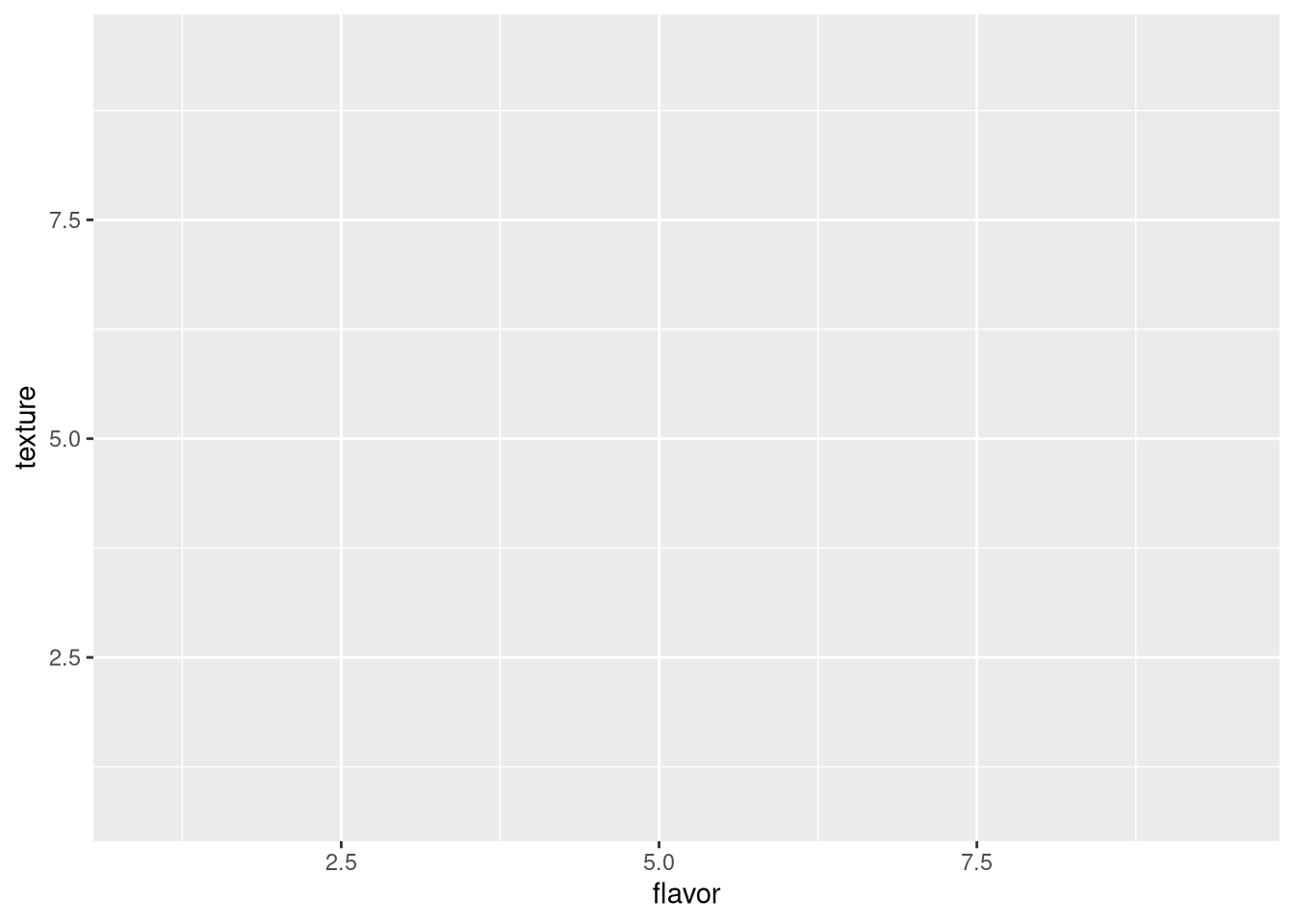
Figure 3.1: Scatter plot of cheese sample flavor v. texture scores, with no geometry specified
aes() are ggplot aesthetics parameters that depend on the chart type. Typically,
x is the quantity or category to plot along the horizontal axis,
y is the quantity or category to plot along the vertical axis,
color determines the color coding for individual data (or shape outlines),
size and shape determine their size and shape,
and fill determines the color coding for shapes representing combined data.
There are many others.
However, note that ggplot() only draws the chart itself, with no data. To draw the data, we must specify their geometry, which for a scatter plot is geom_point().
pdf("pdf/cheese-scatter-plot.pdf")
ggplot(my_data_frame, aes(x = flavor, y = texture)) +
  geom_point()
dev.off()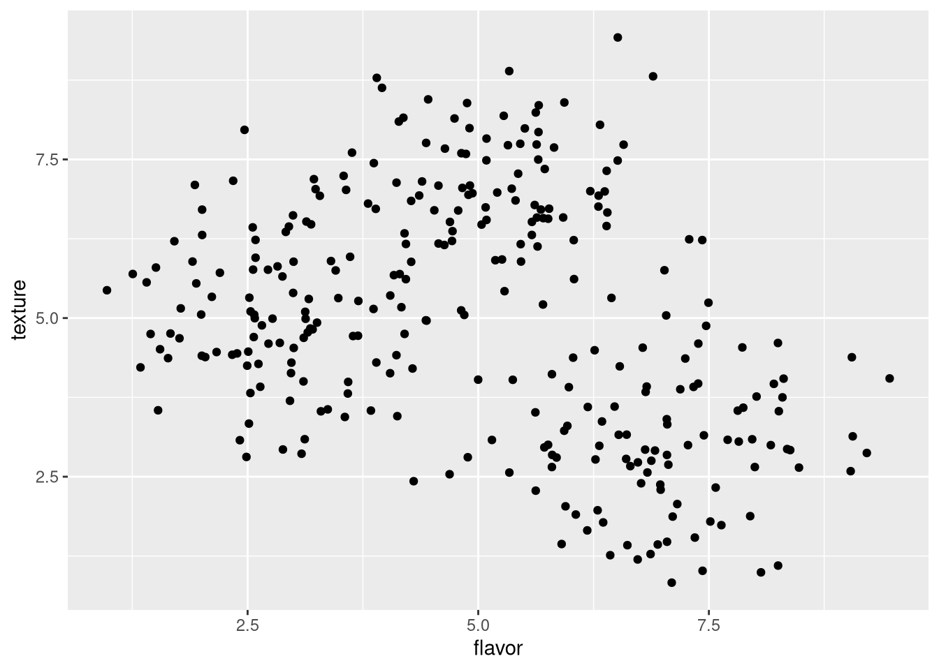
Figure 3.2: Scatter plot of cheese sample flavor v. texture scores
Now we can see the data points, but cannot distinguish which points correspond to which cheese. We can color-code the points by cheese to reveal the clusters corresponding to each cheese.
pdf("pdf/cheese-scatter-plot.pdf")
ggplot(my_data_frame, aes(x = flavor, y = texture, color = cheese)) +
  geom_point()
dev.off()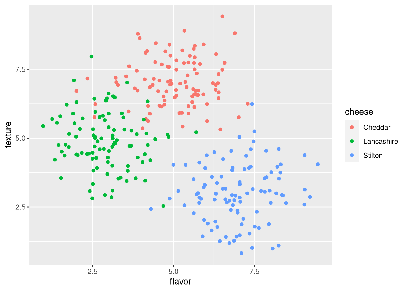
Figure 3.3: Scatter plot of cheese sample flavor v. texture scores, colored by cheese
Note that aesthetics set in later additions to the ggplot override earlier ones. In the following example, the random colors set in geom_point() override those corresponding to the cheese in ggplot().
pdf("pdf/cheese-scatter-plot-random-colors.pdf")
ggplot(my_data_frame, aes(x = flavor, y = texture, color = cheese)) +
  geom_point(color = sample(c("orange", "magenta", "cyan"), nrow(my_data_frame), replace = TRUE))
dev.off()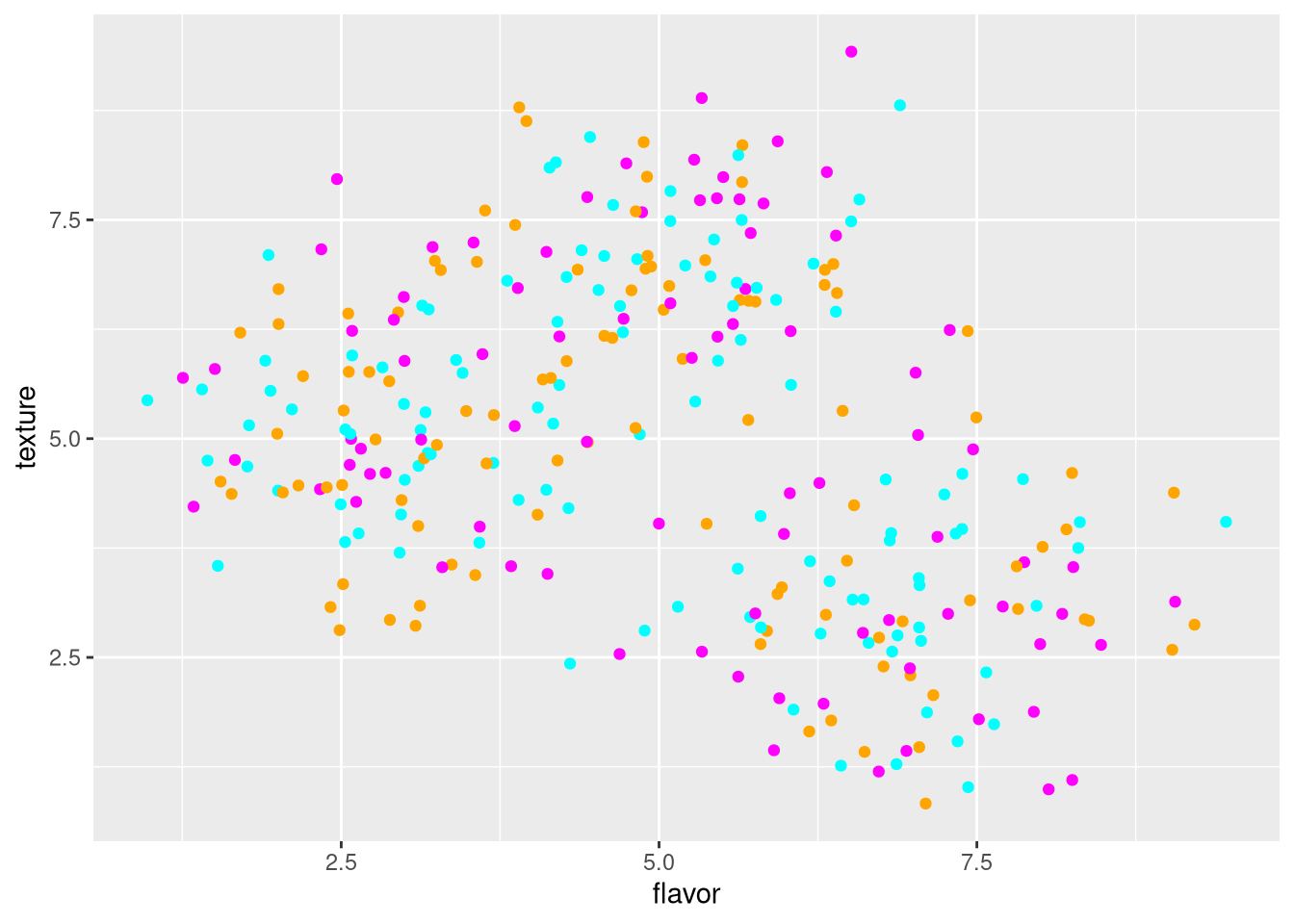
Figure 3.4: Scatter plot of cheese sample flavor v. texture scores, with color overridden
3.6.2 Bar plot
A bar plot shows counts of categorical data, in this case the number of cheese samples.
pdf("pdf/cheese-bar-plot.pdf")
ggplot(my_data_frame[my_data_frame$flavor > 5, ], aes(x = cheese, fill = cheese)) +
  geom_bar()
dev.off()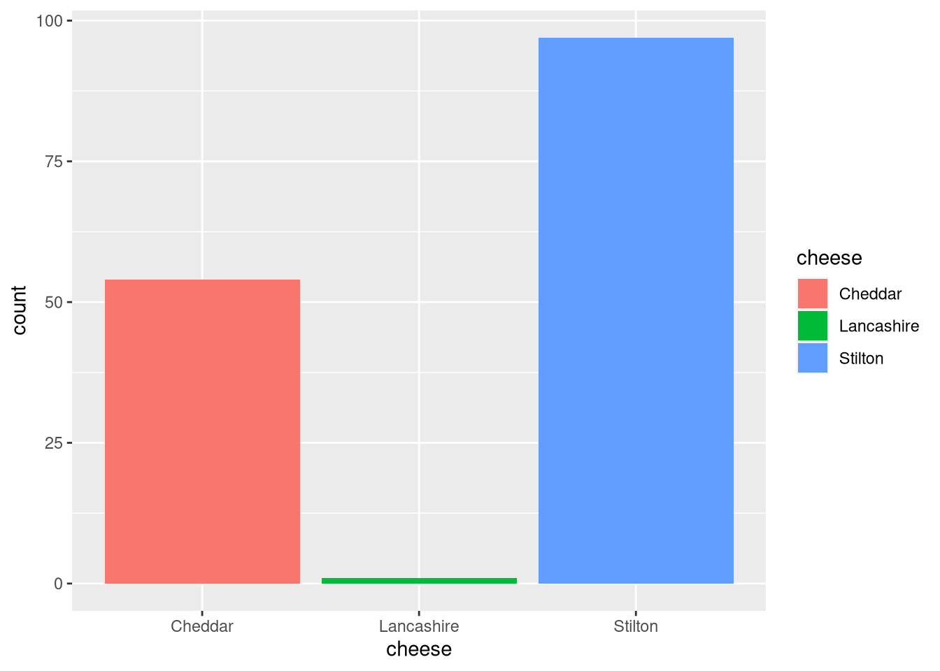
Figure 3.5: Bar plot of cheese samples with flavor score 5 or higher
3.6.3 Histogram
A histogram is similar to a bar plot, but for numeric data binned into artificial categories (instead of intrinsically categorical data). The default is to create 30 bins between the minimum and maximum values.
pdf("pdf/cheese-bar-plot.pdf")
ggplot(my_data_frame, aes(x = flavor)) +
  geom_histogram(color = "black", fill = "red")
dev.off()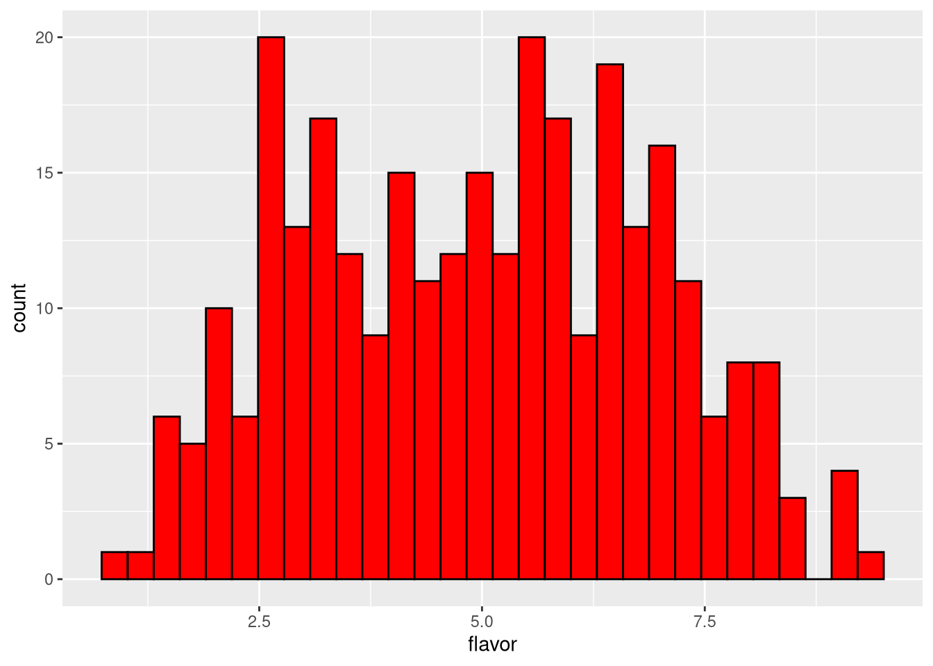
Figure 3.6: Histogram of cheese flavor scores, default of 30 bins
But we can specify the number of bins between the extreme values,
pdf("pdf/cheese-bar-plot.pdf")
ggplot(my_data_frame, aes(x = flavor)) +
  geom_histogram(bins = 10, color = "black", fill = "green")
dev.off()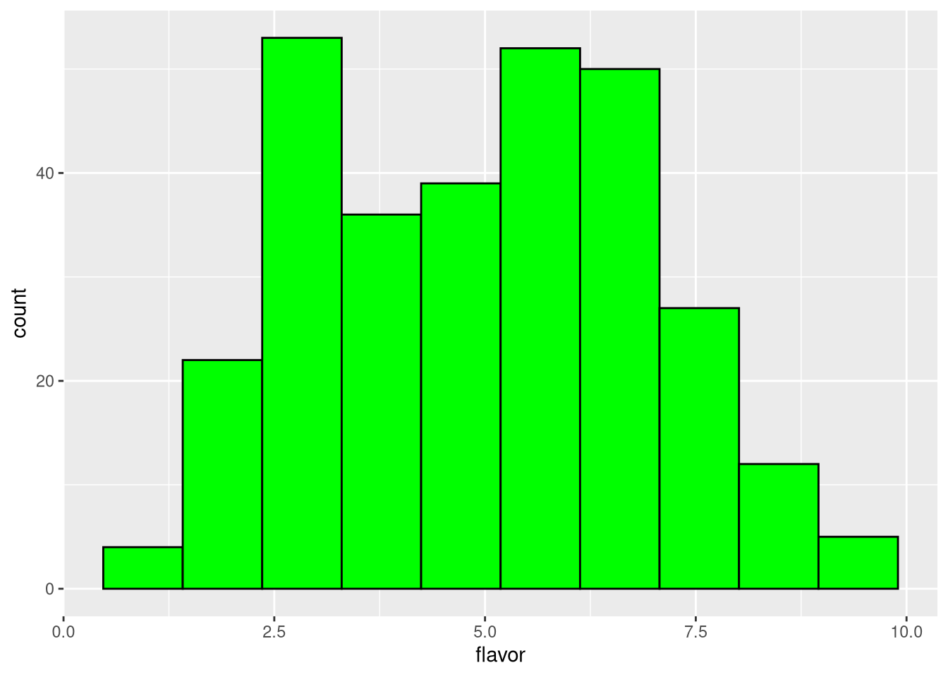
Figure 3.7: Histogram of cheese flavor scores, 10 bins
Or explicitly set the width of each bin.
pdf("pdf/cheese-bar-plot.pdf")
ggplot(my_data_frame, aes(x = flavor)) +
  geom_histogram(binwidth = 0.1, color = "black", fill = "blue")
dev.off()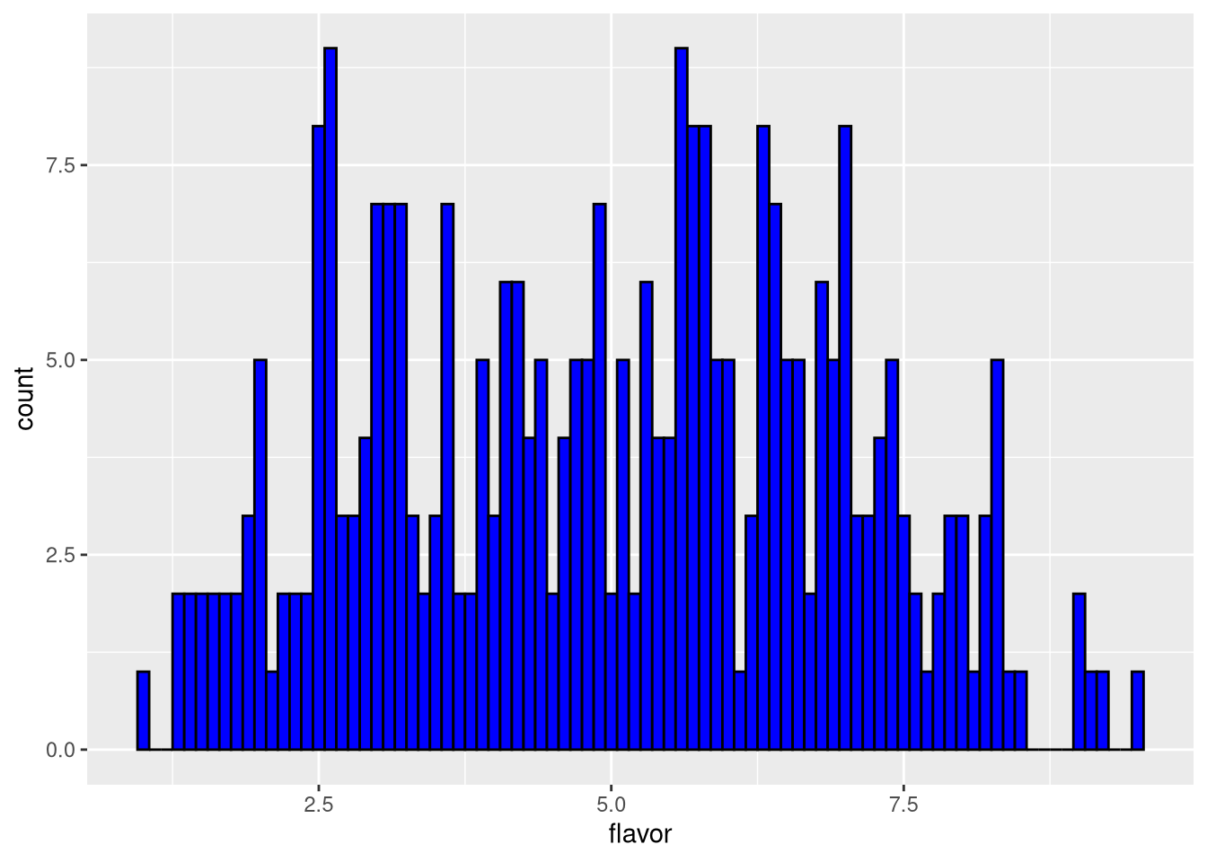
Figure 3.8: Histogram of cheese flavor scores, bin width = 0.1
3.6.4 Box-and-whiskers plot
A box-and-whiskers (or just box) plot summarizes the distribution of numeric data in cases where there are too many data points to visualize on a scatter plot, as regions of moderate and high data density would both appear full or cluttered. Instead, it shows a rectangular box whose top and bottom are at different quantiles (typically 75% and 25%), with a horizontal line at the median (50%) and vertical lines extending to more extreme quantiles (typically 95% and 5%). Data points outside this range may be shown as individual outliers. This example is a box plot of the flavor values of each cheese.
pdf("pdf/cheese-box-plot.pdf")
ggplot(my_data_frame, aes(x = cheese, y = flavor, fill = cheese)) +
  geom_boxplot()
dev.off()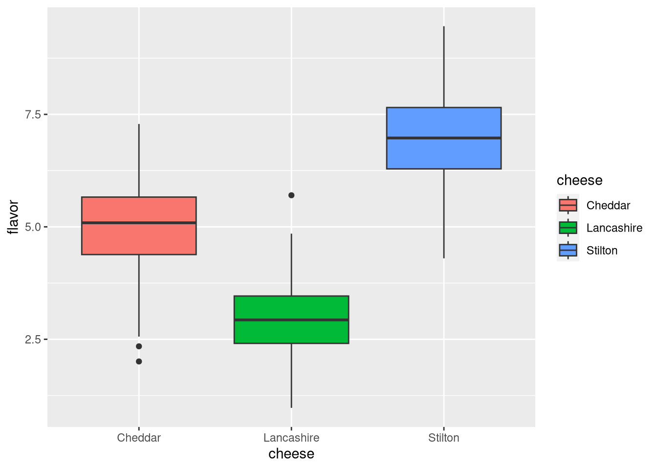
Figure 3.9: Box plot of cheese flavor scores
3.6.5 Violin plot
Like the box plot, a violin plot is another way to visualize dense data. The curve is constructed by centering a small symmetric “blip” (technically a probability density function, for example a normal distribution) at the value of each data point, and adding all of the blips together, resulting in a wider bulge where the data are denser. This example is a violin plot of the texture values of each cheese.
pdf("pdf/cheese-violin-plot.pdf")
ggplot(my_data_frame, aes(x = cheese, y = texture, fill = cheese)) +
  geom_violin()
dev.off()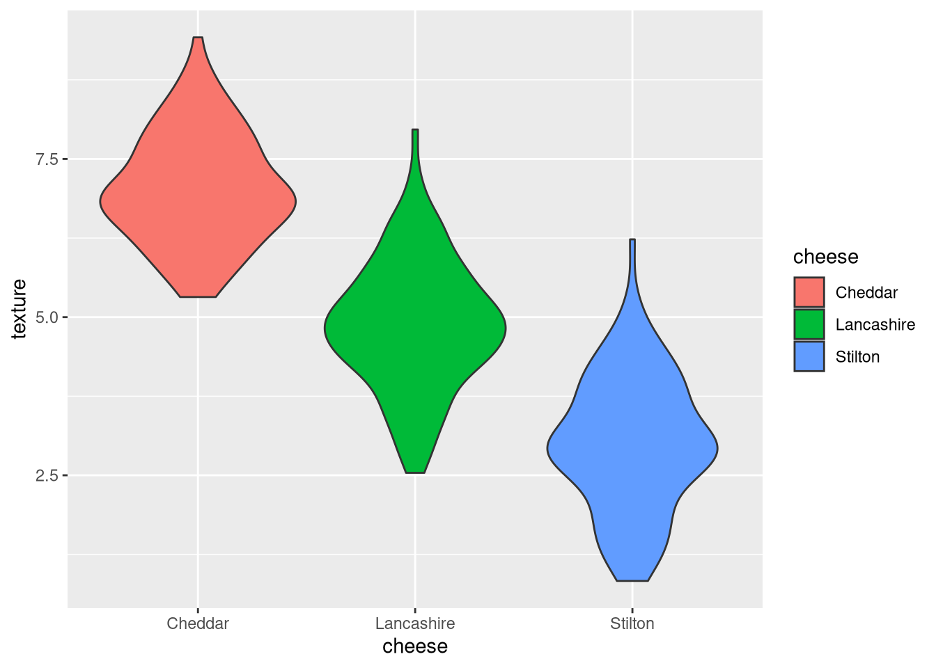
Figure 3.10: Violin plot of cheese texture scores
3.6.6 Heatmap
A heatmap shows the value or “height” of two-dimensional data as a color, similar to a low-resolution topological map.
# data frame representing an n x n grid of random values
set.seed(42)
n <- 16
heatmap_data_frame <- data.frame(
  x = rep(1:n, each = n),
  y = rep(1:n, times = n),
  value = runif(n*n, min = -1, max = 1)
)

pdf("pdf/heatmap-squares.pdf")
ggplot(heatmap_data_frame, aes(x, y)) +
  geom_tile(aes(fill = value)) +
  scale_fill_gradient2(low = "darkblue", mid = "white", high = "darkred") +
  coord_fixed() # sets aspect ratio to 1
dev.off()

pdf("pdf/heatmap-dots.pdf")
ggplot(heatmap_data_frame, aes(x, y)) +
  geom_point(aes(color = value, size = abs(value))) +
  scale_color_gradient2(low = "darkblue", mid = "white", high = "darkred") +
  coord_fixed() +
  theme_bw() +
  theme(legend.position = "none")
dev.off()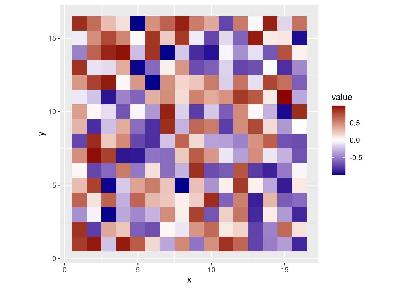
Figure 3.11: Heatmap using squares
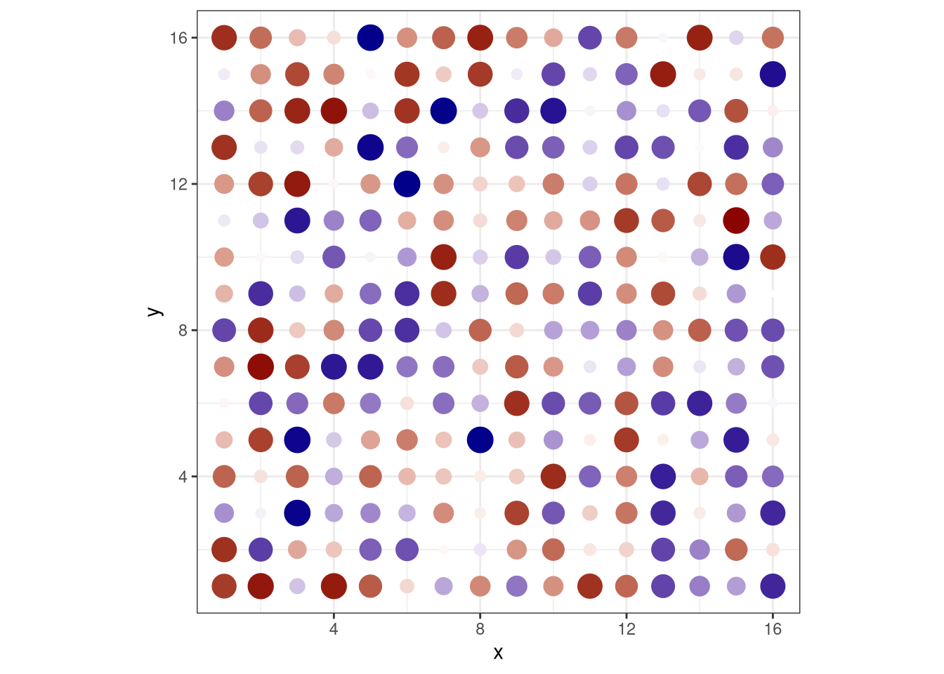
Figure 3.12: Heatmap using dots
3.7 Best practices
3.7.2 Code standards
Coding standards enforce consistency and readability across your code base, affecting everything from the choice of variable names to the structural organization of large, complex data sets.
The R/Tidyverse style guide is one example.
3.7.3 Pipes
One aspect of code readability involves how to chain functions together. Suppose we have three functions that we want to apply sequentially to our data, first f1(), then f2(), then f3().
f1 <- function(x) { x^2 }
f2 <- function(y) { y - 2 }
f3 <- function(z) { 3*z }
The usual way is to nest the functions.
x <- 4
# the following is equivalent to
# y <- f1(x)
# z <- f2(y)
# f3(z)
f3(f2(f1(x)))
## [1] 42However, this can be confusing to someone trying to figure out what the code does, as they have to un-nest the functions in their mind and realize that f1() is applied before f2() and f3(), though they appear in reverse order.
A better way is to use the %>% (“pipe”) operator from the magrittr package, which passes the data on its left as an argument to the function on its right. As the order of writing and execution are the same, the code is easier to understand.
library(magrittr)
x %>% f1() %>% f2() %>% f3()
## [1] 42Beginning with R 4.1, base R has its own pipe operator, |>.
x |> f1() |> f2() |> f3()## [1] 42For simple functions like ours, this behaves more or less like %>%, but %>% has some extra functionality that is beyond the scope of this introduction. Refer to the |> and %>% documentation for more details.
3.7.4 Metadata
It is good form to wrap your data in a unified package containing supplementary information (metadata) about them and how they were acquired or assembled from different sources. For example, your single cell data may consist of batches from separate experiments run on different days and under different conditions. The single cell data structures we will use in subsequent chapters are already designed this way. Such integrated data sets are also known as rich data.
In this simple example, we combine our cheese tasting data frame with the original vector of cheeses we might have considered tasting (had they been available in the shop), and add information about the combined data set. We do so using nested lists with named elements,
my_data <- list(
  data = my_data_frame,
  superset = british_cheeses,
  metadata = list(
    name = "Cheese tasting data",
    description = "Flavor and texture scores for selected British cheeses",
    author = "Henry Wensleydale",
    date = "2022-03-04"
  )
)
str(my_data)
## List of 3
## $ data :'data.frame': 300 obs. of 4 variables:
## ..$ guest_id: int [1:300] 1 1 1 2 2 2 3 3 3 4 ...
## ..$ cheese : chr [1:300] "Cheddar" "Lancashire" "Stilton" "Cheddar" ...
## ..$ flavor : num [1:300] 6.37 4.2 5 4.44 4.04 ...
## ..$ texture : num [1:300] 7 6.33 4.03 7.76 4.13 ...
## $ superset: chr [1:12] "Caerphilly" "Cheddar" "Cheshire" "Dorset Blue Vinney" ...
## $ metadata:List of 4
## ..$ name : chr "Cheese tasting data"
## ..$ description: chr "Flavor and texture scores for selected British cheeses"
## ..$ author : chr "Henry Wensleydale"
## ..$ date : chr "2022-03-04"With all of the data in one place, future users can easily navigate through the named elements using the $ operator, find answers to questions about the data provenance, and can determine other information such as which cheeses were not tasted.
# Can you summarize this data set while standing on one foot?
my_data$metadata$description
## [1] "Flavor and texture scores for selected British cheeses"# Which cheeses were (in theory) available, but not tasted?
setdiff(my_data$superset, my_data$data$cheese)## [1] "Caerphilly" "Cheshire" "Dorset Blue Vinney"
## [4] "Double Gloucester" "Red Leicester" "Red Windsor"
## [7] "Sage Derby" "Wensleydale" "White Stilton"A more advanced way is to use S4 classes, which have “slots” for different data elements. In the Seurat chapter, we will see that the Seurat data structure is an example of an S4 object.
3.7.5 Tidy data
We mentioned earlier how data frames should be organized so that each row is an observation and each column is a variable. This is the essence of tidy data, first described in this article:
Wickham, Tidy Data, J. Statistical Software 59 (10), August 2014.
Many R packages (such as ggplot2) expect data to be in a tidy format, and may not function as expected if they are not.
Worrying about whether your data are sufficiently tidy gets into the philosophical question of “What even is an observation?“ Consider our cheese tasting data frame, my_data_frame.
head(my_data_frame)## guest_id cheese flavor texture
## 1 1 Cheddar 6.370958 6.995379
## 2 1 Lancashire 4.200965 6.334913
## 3 1 Stilton 4.999071 4.029141
## 4 2 Cheddar 4.435302 7.760242
## 5 2 Lancashire 4.044751 4.130728
## 6 2 Stilton 7.333777 3.914775dim(my_data_frame)## [1] 300 4Each row is a guest’s observation of both scores (flavor and texture) for one cheese. But what if we want to consider the flavor and texture scores as independent observations? We would have to split each row into two rows, one with only the flavor score and one with only the texture score. Fortunately there is a function to do so, called pivot_longer() because it makes the data frame a “longer” table (with more rows and fewer columns). This comes from the tidyr package, so we need to load that first.
library(tidyr)my_data_frame_long <- pivot_longer(my_data_frame, cols = c("flavor", "texture"), names_to = "quality", values_to = "score")
head(my_data_frame_long)## # A tibble: 6 × 4
## guest_id cheese quality score
## <int> <chr> <chr> <dbl>
## 1 1 Cheddar flavor 6.37
## 2 1 Cheddar texture 7.00
## 3 1 Lancashire flavor 4.20
## 4 1 Lancashire texture 6.33
## 5 1 Stilton flavor 5.00
## 6 1 Stilton texture 4.03dim(my_data_frame_long)## [1] 600 4As expected, my_data_frame_long has twice as many rows as my_data_frame.
On the other hand, what if we define the observation as each guest’s complete tasting experience? We would have to combine the scores for all cheeses into a single row with more score columns, making the data frame a “wider” table. The analogous function is pivot_wider(),
my_data_frame_wide <- pivot_wider(my_data_frame, names_from = "cheese", names_glue = "{cheese}_{.value}", values_from = c("flavor", "texture"))
head(my_data_frame_wide)
## # A tibble: 6 × 7
## guest_id Cheddar_flavor Lancashire_flavor Stilton_flavor Cheddar_texture
## <int> <dbl> <dbl> <dbl> <dbl>
## 1 1 6.37 4.20 5.00 7.00
## 2 2 4.44 4.04 7.33 7.76
## 3 3 5.36 2.00 8.17 7.04
## 4 4 5.63 4.85 9.06 7.74
## 5 5 5.40 2.33 5.62 6.85
## 6 6 4.89 3.11 5.85 6.94
## # ℹ 2 more variables: Lancashire_texture <dbl>, Stilton_texture <dbl>dim(my_data_frame_wide)## [1] 100 7As expected, my_data_frame_wide has only one third as many rows as my_data_frame, and more columns.
As we see from our longer and wider examples, there is not necessarily a well defined tidyness for a given data set. You have to tailor yours to your needs.
3.8 Quitting R
When you are done with your session, enter q() to quit R and return to the Linux command line.
3.9 Further resources
The main R site is the Comprehensive R Archive Network (CRAN). Much more information about obtaining and using R is available there.
RStudio is an integrated development environment for R, with both desktop and server versions.
One advantage of running R or RStudio on your own computer is the ability to display graphics in their own window. This eliminates the need to save them to a PDF or image file as required on the NCGR server.
Data tidying with tidyr cheat sheet
Differences between the base R and magrittr pipes
3.9.1 R books
Chang, R Graphics Cookbook
Grolemund and Wickham, R for Data Science
Long and Teetor, R Cookbook: Proven Recipes for Data Analysis, Statistics, and Graphics
Wickham, Navarro, and Pedersen, ggplot2: Elegant Graphics for Data Analysis
3.7.1 Comments
Comments are lines in your code starting with ‘#’, intended for description rather than execution. It is a good idea to divide your code into functional blocks preceded by a comment, so that future programmers can better understand what it does.