5 Quality Control
Single cell datasets typically include data from dead or weakly expressing cells as well as accidental doublet or multiplet cells. These can introduce noise or spurious clusters into our results, so it is important to eliminate them before further analysis. In this chapter, we will learn about different quality control methods.
library(SingleCellExperiment)
library(scater)
library(ggplot2)
We begin by reading in our saved data (if necessary) and inspecting the row and column metadata.
# Do not run - depends on workshop timing
# my_SCE <- readRDS("data/my_SCE-03.rds")

head(rowData(my_SCE))
## DataFrame with 6 rows and 3 columns
## ID Symbol Type
## <character> <character> <character>
## AT1G01010 AT1G01010 AT1G01010 Gene Expression
## AT1G01020 AT1G01020 AT1G01020 Gene Expression
## AT1G03987 AT1G03987 AT1G03987 Gene Expression
## AT1G01030 AT1G01030 AT1G01030 Gene Expression
## AT1G01040 AT1G01040 AT1G01040 Gene Expression
## AT1G03993 AT1G03993 AT1G03993 Gene Expressionhead(colData(my_SCE))## DataFrame with 6 rows and 5 columns
## Sample Barcode sizeFactor
## <character> <character> <numeric>
## AAACCCACACGCGCAT-1 data/filtered_featur.. AAACCCACACGCGCAT-1 0.764455
## AAACCCACAGAAGTTA-1 data/filtered_featur.. AAACCCACAGAAGTTA-1 0.872851
## AAACCCACAGACAAAT-1 data/filtered_featur.. AAACCCACAGACAAAT-1 1.576417
## AAACCCACATTGACAC-1 data/filtered_featur.. AAACCCACATTGACAC-1 2.051818
## AAACCCAGTAGCTTTG-1 data/filtered_featur.. AAACCCAGTAGCTTTG-1 0.415850
## AAACCCAGTCCAGTTA-1 data/filtered_featur.. AAACCCAGTCCAGTTA-1 0.366336
## total_counts num_genes_expressed
## <numeric> <integer>
## AAACCCACACGCGCAT-1 2285 1382
## AAACCCACAGAAGTTA-1 2609 1525
## AAACCCACAGACAAAT-1 4712 2606
## AAACCCACATTGACAC-1 6133 3434
## AAACCCAGTAGCTTTG-1 1243 998
## AAACCCAGTCCAGTTA-1 1095 914Recall that the point of single cell analysis is to look for variation between cells. This gives us a clue about which cells to remove. Consider the mean v. variance of gene expression by cell.
mean_counts <- colMeans(counts(my_SCE))
var_counts <- colVars(counts(my_SCE))pdf("pdf/mean-variance.pdf")
ggcells(my_SCE, aes(x = mean_counts, y = var_counts)) +
geom_point(aes(color = "identity"), show.legend = FALSE) +
scale_color_manual(values = "blue")
dev.off()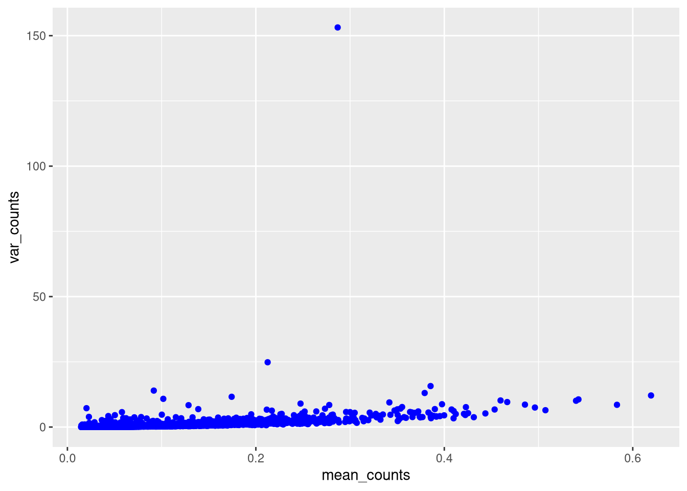
Figure 5.1: Mean v. variance of cell counts
Click for answer
One way is to filter out var_counts > 50 or so, but this removes that point from the data.
A better way is to limit the y axis of the chart, by adding a ylim(min, max) statement.
pdf("pdf/mean-variance-limit-y-axis.pdf")
ggcells(my_SCE, aes(x = mean_counts, y = var_counts)) +
  geom_point(aes(color = "identity"), show.legend = FALSE) +
  scale_color_manual(values = "blue") +
  ylim(0, 25)
dev.off()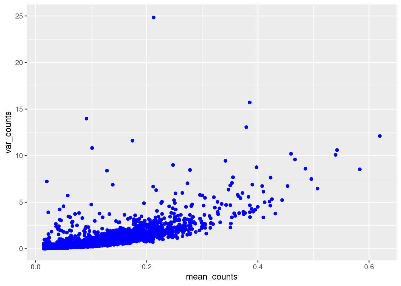
We see that variance generally increases with mean counts (gene expression), so cells with low counts are candidates for removal.
5.1 Built-in functions for basic QC metrics
We can begin by computing basic QC metrics, using functions from package scuttle.
my_SCE <- addPerCellQCMetrics(my_SCE)
head(colData(my_SCE))
## DataFrame with 6 rows and 8 columns
## Sample Barcode sizeFactor
## <character> <character> <numeric>
## AAACCCACACGCGCAT-1 data/filtered_featur.. AAACCCACACGCGCAT-1 0.764455
## AAACCCACAGAAGTTA-1 data/filtered_featur.. AAACCCACAGAAGTTA-1 0.872851
## AAACCCACAGACAAAT-1 data/filtered_featur.. AAACCCACAGACAAAT-1 1.576417
## AAACCCACATTGACAC-1 data/filtered_featur.. AAACCCACATTGACAC-1 2.051818
## AAACCCAGTAGCTTTG-1 data/filtered_featur.. AAACCCAGTAGCTTTG-1 0.415850
## AAACCCAGTCCAGTTA-1 data/filtered_featur.. AAACCCAGTCCAGTTA-1 0.366336
## total_counts num_genes_expressed sum detected
## <numeric> <integer> <numeric> <integer>
## AAACCCACACGCGCAT-1 2285 1382 2285 1382
## AAACCCACAGAAGTTA-1 2609 1525 2609 1525
## AAACCCACAGACAAAT-1 4712 2606 4712 2606
## AAACCCACATTGACAC-1 6133 3434 6133 3434
## AAACCCAGTAGCTTTG-1 1243 998 1243 998
## AAACCCAGTCCAGTTA-1 1095 914 1095 914
## total
## <numeric>
## AAACCCACACGCGCAT-1 2285
## AAACCCACAGAAGTTA-1 2609
## AAACCCACAGACAAAT-1 4712
## AAACCCACATTGACAC-1 6133
## AAACCCAGTAGCTTTG-1 1243
## AAACCCAGTCCAGTTA-1 1095addPerCellQCMetrics() created three new columns: sum, detected, and total. Note that sum and total are identical to our handmade total_counts, and detected is the same as our num_genes_expressed, so we may remove our two columns from the previous chapter.
my_SCE$total_counts <- my_SCE$num_genes_expressed <- NULL
head(colData(my_SCE))
## DataFrame with 6 rows and 6 columns
## Sample Barcode sizeFactor
## <character> <character> <numeric>
## AAACCCACACGCGCAT-1 data/filtered_featur.. AAACCCACACGCGCAT-1 0.764455
## AAACCCACAGAAGTTA-1 data/filtered_featur.. AAACCCACAGAAGTTA-1 0.872851
## AAACCCACAGACAAAT-1 data/filtered_featur.. AAACCCACAGACAAAT-1 1.576417
## AAACCCACATTGACAC-1 data/filtered_featur.. AAACCCACATTGACAC-1 2.051818
## AAACCCAGTAGCTTTG-1 data/filtered_featur.. AAACCCAGTAGCTTTG-1 0.415850
## AAACCCAGTCCAGTTA-1 data/filtered_featur.. AAACCCAGTCCAGTTA-1 0.366336
## sum detected total
## <numeric> <integer> <numeric>
## AAACCCACACGCGCAT-1 2285 1382 2285
## AAACCCACAGAAGTTA-1 2609 1525 2609
## AAACCCACAGACAAAT-1 4712 2606 4712
## AAACCCACATTGACAC-1 6133 3434 6133
## AAACCCAGTAGCTTTG-1 1243 998 1243
## AAACCCAGTCCAGTTA-1 1095 914 1095(Our data are from a single experiment. For a SingleCellExperiment object containing data from multiple experiments, sum is the sum of cell counts in each experiment, and total is across all experiments.)
And for genes,
my_SCE <- addPerFeatureQCMetrics(my_SCE)
head(rowData(my_SCE))
## DataFrame with 6 rows and 5 columns
## ID Symbol Type mean detected
## <character> <character> <character> <numeric> <numeric>
## AT1G01010 AT1G01010 AT1G01010 Gene Expression 0.10276817 8.442907
## AT1G01020 AT1G01020 AT1G01020 Gene Expression 0.23131488 18.529412
## AT1G03987 AT1G03987 AT1G03987 Gene Expression 0.00000000 0.000000
## AT1G01030 AT1G01030 AT1G01030 Gene Expression 0.01885813 1.747405
## AT1G01040 AT1G01040 AT1G01040 Gene Expression 0.47439446 33.166090
## AT1G03993 AT1G03993 AT1G03993 Gene Expression 0.00017301 0.017301addPerFeatureQCMetrics() created two new columns: mean and detected. These are the mean counts and percentage of observations above a threshold (0 by default).
5.2 Thresholds
Once we have computed relevant metrics, we can use them to filter out low-quality cells. We can either set a fixed threshold for individual metrics by exploratory data analysis, or decide on an adaptive threshold using statistical considerations.
5.2.1 Fixed thresholds
We can estimate fixed thresholds for the cell counts and number of expressed genes by looking at their histograms,
sum_threshold <- 1000
detected_threshold <- 750pdf("pdf/histogram-cell-counts.pdf")
ggcells(my_SCE, aes(x = sum)) +
geom_histogram(binwidth = 200, color = "black", fill = "cyan") +
geom_vline(xintercept = sum_threshold, col = "red", lty = "dashed")
dev.off()
pdf("pdf/histogram-cell-num-genes-expressed.pdf")
ggcells(my_SCE, aes(x = detected)) +
geom_histogram(binwidth = 100, color = "black", fill = "green") +
geom_vline(xintercept = detected_threshold, col = "red", lty = "dashed")
dev.off()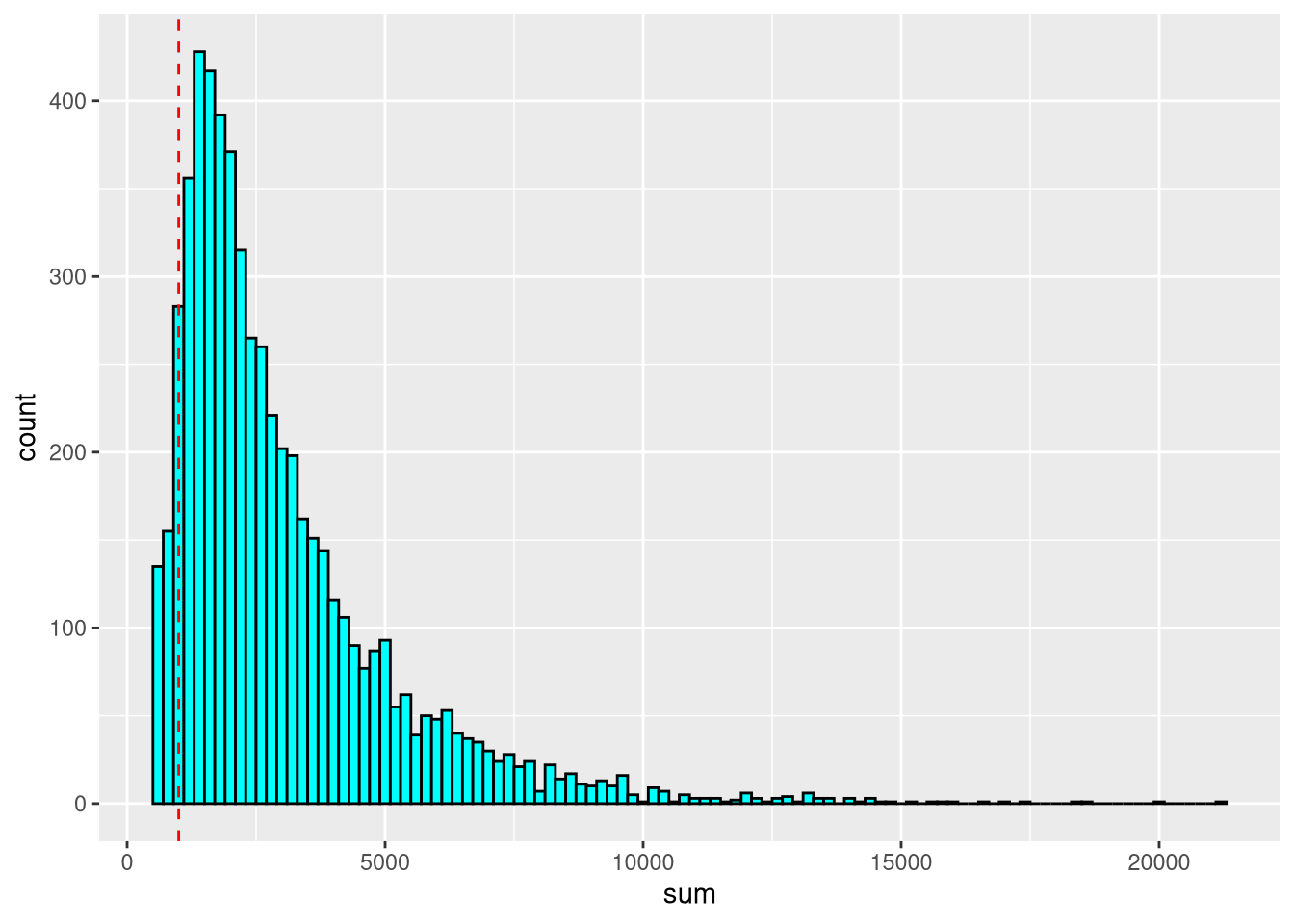
Figure 5.2: Histogram of cell counts
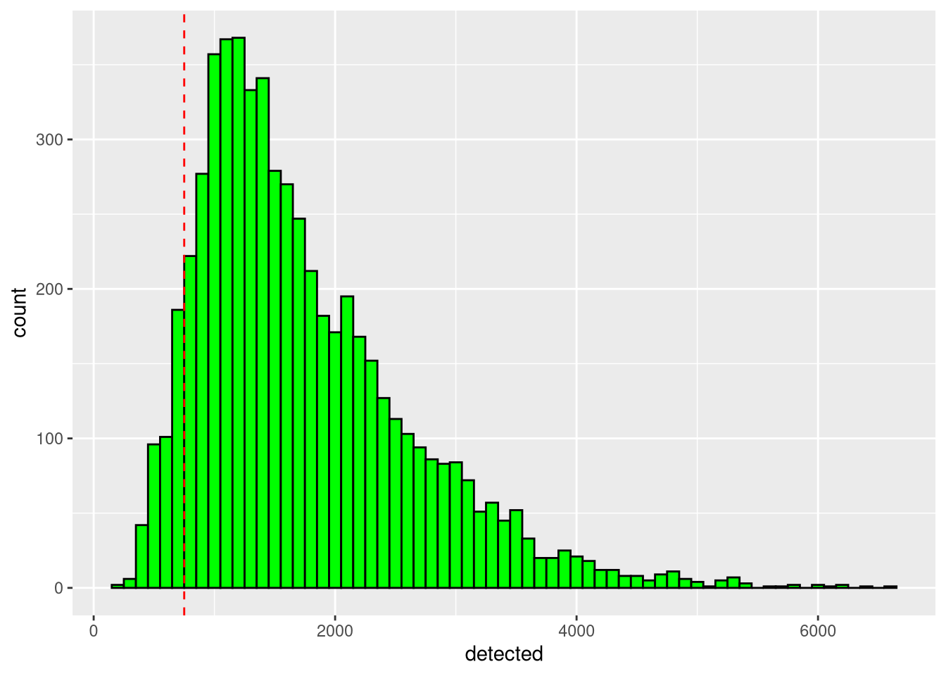
Figure 5.3: Histogram of cell number of expressed genes
5.2.2 Adaptive thresholds
The functions isOutlier() and perCellQCFilters() (from the scuttle package) automatically determine outliers (for one or all cell quality control metrics, respectively), as a proxy for low-quality cells. The optional nmads argument (default = 3) controls how far a data point must be from the median (in median absolute deviations) to be considered an outlier.
colData(my_SCE) <- cbind(colData(my_SCE), perCellQCFilters(my_SCE))
head(colData(my_SCE))
## DataFrame with 6 rows and 9 columns
## Sample Barcode sizeFactor
## <character> <character> <numeric>
## AAACCCACACGCGCAT-1 data/filtered_featur.. AAACCCACACGCGCAT-1 0.764455
## AAACCCACAGAAGTTA-1 data/filtered_featur.. AAACCCACAGAAGTTA-1 0.872851
## AAACCCACAGACAAAT-1 data/filtered_featur.. AAACCCACAGACAAAT-1 1.576417
## AAACCCACATTGACAC-1 data/filtered_featur.. AAACCCACATTGACAC-1 2.051818
## AAACCCAGTAGCTTTG-1 data/filtered_featur.. AAACCCAGTAGCTTTG-1 0.415850
## AAACCCAGTCCAGTTA-1 data/filtered_featur.. AAACCCAGTCCAGTTA-1 0.366336
## sum detected total low_lib_size
## <numeric> <integer> <numeric> <outlier.filter>
## AAACCCACACGCGCAT-1 2285 1382 2285 FALSE
## AAACCCACAGAAGTTA-1 2609 1525 2609 FALSE
## AAACCCACAGACAAAT-1 4712 2606 4712 FALSE
## AAACCCACATTGACAC-1 6133 3434 6133 FALSE
## AAACCCAGTAGCTTTG-1 1243 998 1243 FALSE
## AAACCCAGTCCAGTTA-1 1095 914 1095 FALSE
## low_n_features discard
## <outlier.filter> <logical>
## AAACCCACACGCGCAT-1 FALSE FALSE
## AAACCCACAGAAGTTA-1 FALSE FALSE
## AAACCCACAGACAAAT-1 FALSE FALSE
## AAACCCACATTGACAC-1 FALSE FALSE
## AAACCCAGTAGCTTTG-1 FALSE FALSE
## AAACCCAGTCCAGTTA-1 FALSE FALSEsum(my_SCE$low_lib_size)## [1] 0sum(my_SCE$low_n_features)## [1] 4sum(my_SCE$discard)## [1] 4pdf("pdf/adaptive-qc.pdf")
plotColData(my_SCE, "detected", "sum", colour_by = "discard")
dev.off()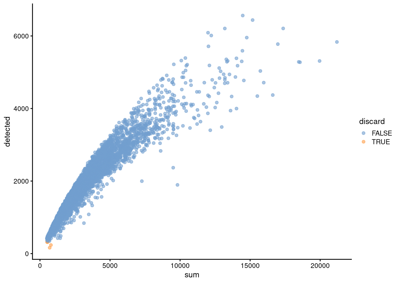
Figure 5.4: Cell counts v. number of expressed genes, showing outliers from adaptive-threshold QC to discard
This adds three columns of metadata, low_lib_size, low_n_features, and discard, though it is possible to have outliers on the high end of the distribution as well.
There are only 4 discards in my_SCE, all of which are outliers in the detected (number of expressed genes) column and none in the sum column (cell counts).
Click for answer
qcf_2_mads <- perCellQCFilters(my_SCE, nmads = 2)
sum(qcf_2_mads$low_lib_size)
## [1] 90sum(qcf_2_mads$low_n_features)## [1] 141sum(qcf_2_mads$discard)## [1] 141detected and 90 also having low sum.
5.2.3 Removing genes
We may also eliminate genes, for example those for mitochondrial or ribosomal proteins. In our dataset, note that the gene names depend on their origin in the Arabidopsis thaliana genome. Those beginning with “AT1” through “AT5” are from chromosomes 1-5, those with “ATC” or “ATM” are from chloroplast and mitochondrial RNA, and those with “ENSRNA” are non-protein coding genes.
gene_prefix <- substring(rowData(my_SCE)$ID, 1, 3)
sort(unique(gene_prefix))
## [1] "AT1" "AT2" "AT3" "AT4" "AT5" "ATC" "ATM" "ENS"We may eliminate the chloroplast, mitochondrial, and RNA genes as they do not contribute to our desired biological signal.
undesired_gene_prefixes <- c("ATC", "ATM", "ENS")
sum(gene_prefix %in% undesired_gene_prefixes)
## [1] 1670This will remove 1670 genes.
5.3 Doublet detection
We would also like to eliminate doublets. The computeDoubletDensity() function (from package scDblFinder) creates a score for each cell that is the average ratio (across a simulation) of the density of simulated doublets containing that cell to the density of the individual cells.
library(scDblFinder)
library(BiocSingular)

set.seed(42)
my_SCE$doublet_score <- computeDoubletDensity(my_SCE)
To determine a plausible doublet score threshold, we make a violin plot of the doublet scores.
pdf("pdf/doublet-scores.pdf")
ggcells(my_SCE, aes(x = Sample, y = doublet_score)) +
  geom_violin(fill = 'blue')
dev.off()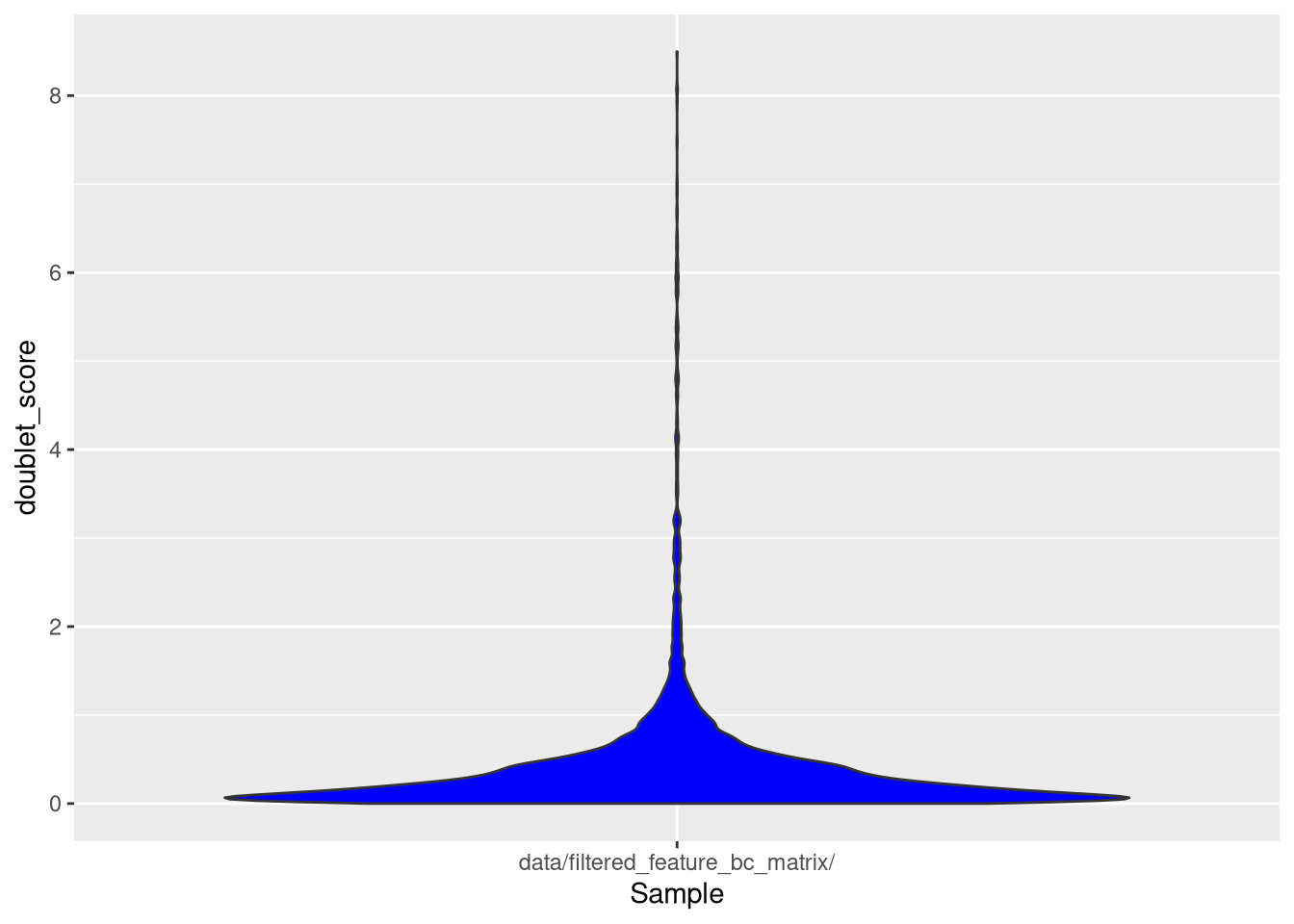
Figure 5.5: Violin plot of doublet scores
Let’s set an arbitrary threshold of 1.9.
doublet_score_threshold <- 1.9
my_SCE$probable_doublet <- (my_SCE$doublet_score > doublet_score_threshold)pdf("pdf/doublet-score-threshold.pdf")
plotColData(my_SCE, "doublet_score", colour_by = "probable_doublet")
dev.off()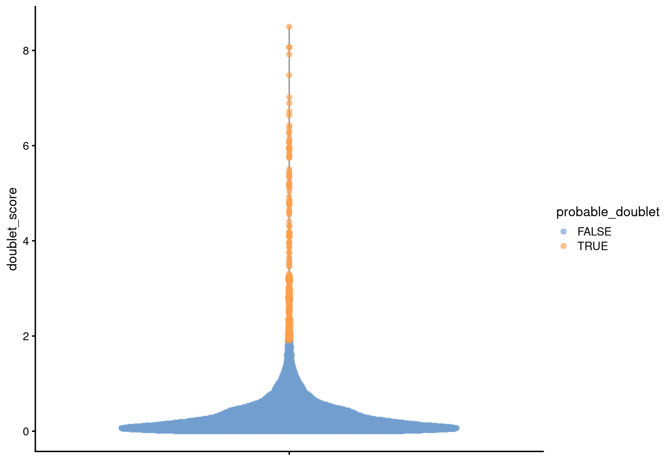
Figure 5.6: Cells to discard due to high doublet score
5.4 Quality-controlled dataset
Finally, we can put all this together and create a smaller, quality-controlled dataset my_SCE_qc. We remove any cells that are discard candidates by either adaptive or fixed thresholds (low counts or number of expressed genes) or high doublet score, and any genes that are not expressed in any cell.
sum(my_SCE$sum < sum_threshold)## [1] 422sum(my_SCE$detected < detected_threshold)## [1] 432sum(my_SCE$probable_doublet)## [1] 198my_SCE$discard <- (my_SCE$discard | my_SCE$sum < sum_threshold | my_SCE$detected < detected_threshold | my_SCE$probable_doublet) # logical vector indicating which cells to discard
sum(my_SCE$discard)## [1] 687pdf("pdf/fixed-threshold-qc.pdf")
plotColData(my_SCE, "detected", "sum", colour_by = "discard")
dev.off()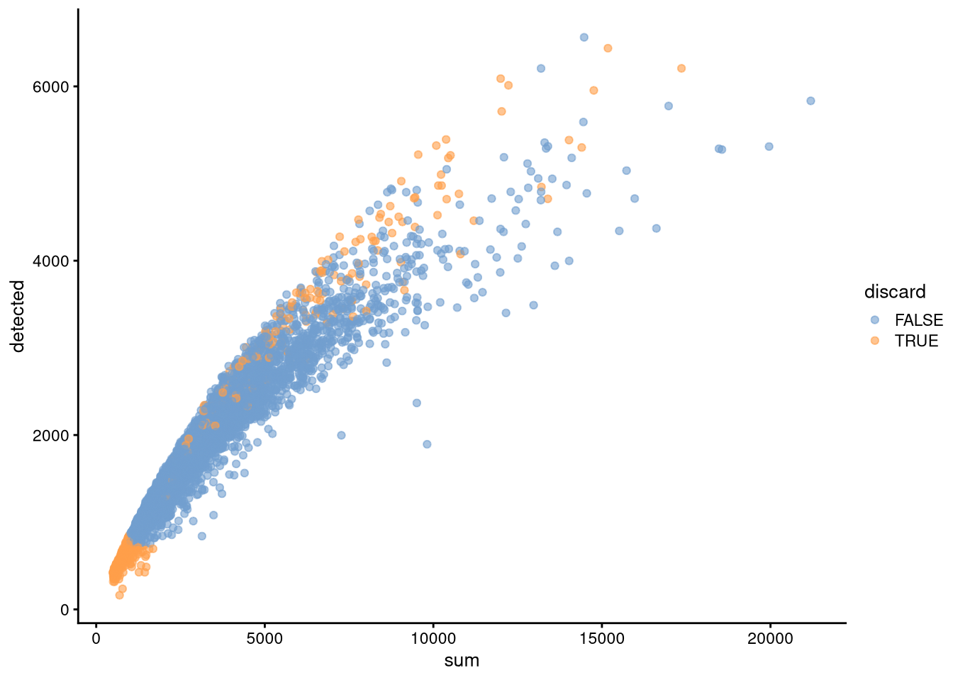
Figure 5.7: Cell counts v. number of expressed genes, showing cells to discard
genes_to_discard <- (gene_prefix %in% undesired_gene_prefixes | rowSums(counts(my_SCE)) == 0)
my_SCE_qc <- my_SCE[!genes_to_discard, !my_SCE$discard]
dim(my_SCE_qc)
## [1] 23848 5093Our quality control process removes 10370 genes and 687 cells. In the next chapter, we will use the remaining data to investigate dimensionality reduction.
To save the quality-controlled dataset,
# Do not run - depends on workshop timing
# saveRDS(my_SCE_qc, "data/my_SCE-04.rds")