8 Integration
Integration is the process of combining single cell data from separate experiments into a unified dataset. Conceptually, we try to remove the technical signal due to differences between the datasets, and retain only the biological signal due to their similarities. From a practical perspective, we want to make similar cells from different datasets cluster together, yielding an apples-to-apples comparison. We achieve this by mathematically determining common sources of variation across datasets, and using this information to systematically map the original data into a new shared feature space.
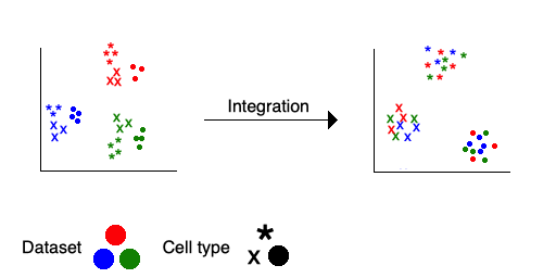
Integration is necessary when you have any of:
- Batch effects from repeated experiments
- Datasets acquired in another laboratory, with different preparation techniques
- Different modalities, such as RNA-seq and ATAC-seq
- Different experimental conditions, such as treated and control cells
In general, it is sensible to perform integration only after looking at each individual dataset.
8.1 Basic Theory
Integration algorithms fall into two general categories: those that compare new data to known cell types from a high-confidence reference dataset (cell atlas), and those that use only common feature and cell data. The former is only valid when the differences in your datasets are mostly due to biological rather than technical factors, while the latter is slower due to the computational complexity of having to compare more pairs of cells. Both assume that there is enough overlap in the feature patterns between datasets to make integration meaningful.
Seurat uses the method of Canonical Correlation Analysis, which falls into the second category (as it does not consider known cell types). CCA somewhat resembles principal component analysis, but works across multiple datasets. Recall that PCA finds the axes of maximum variation (in feature/gene space) within a single dataset, and uses these as a new feature space. Similarly, CCA finds pairs of axes with maximum correlated variation between datasets, and assigns a score to each one. We also identify pairs of cells that are mutual nearest neighbors (anchors) between datasets. From the combination of scores and anchors, we derive corrective vectors to add to each cell’s representation in feature space, shifting the anchors into close alignment and (we hope) correctly clustering the less similar cells as well.
There are many other ways to perform single cell data integration. The 2020 article by Tran et al. (link below) compares 14 of these; Seurat (v3) was one of the top performers, along with Harmony and LIGER.
8.2 Setup
We are going to use Seurat to read and integrate two samples from Farmer et al. (2021). First we load the packages we will need,
library(Seurat)
library(gridExtra)
We also create symbolic links to the data directories, and redefine the cluster colors up front.
if (!file.exists("data4")) system("ln -s /home/data/single-cell-workshop/data-farmer-et-al/sNucRNA-seq_rep4/ data4")
if (!file.exists("data5")) system("ln -s /home/data/single-cell-workshop/data-farmer-et-al/sNucRNA-seq_rep5/ data5")

# Assign display colors for the 21 clusters and 6 superclusters
# (close to those used in Farmer et al.)
cluster_colors <- c(
  "cornflowerblue", "darkblue", "cyan",
  "springgreen", "olivedrab", "chartreuse", "darkgreen",
  "gray", "black", "saddlebrown",
  "slateblue", "purple", "pink", "lightpink3", "hotpink", "darkred",
  "lightsalmon", "orange", "tan", "firebrick1", "indianred"
)
supercluster_colors <- c("blue", "green", "black", "magenta", "red", "orange")
To streamline the process, we define a function that contains a minimal version of the essential code for processing our individual datasets, ending up with PCA and UMAP dimensionality reductions. (At your leisure, you may compare this to the more explicit code in the Seurat chapter.)
# Input: n = the number of the dataset
processNthDataset <- function(n) {
  # Read nth dataset
  dir_data_n <- paste0("data", n)
  my_counts_n <- Read10X(paste0(dir_data_n, "/filtered_feature_bc_matrix/"))
  # Add "_n" to ensure unique cell barcodes for integration
  colnames(my_counts_n) <- paste0(colnames(my_counts_n), "_", n)
  my_seurat_n <- CreateSeuratObject(counts = my_counts_n, project = paste("Dataset", n))

  # Add cluster metadata
  df.clusters_n <- readRDS(paste0(dir_data_n, "/clusters_", n, ".rds"))
  my_seurat_n@meta.data <- merge(my_seurat_n@meta.data, df.clusters_n, by.x = "row.names", by.y = "cell_barcode", all.x = TRUE)
  # It converted row.names(my_seurat@meta.data) to a spurious column called Row.names, so clean up
  row.names(my_seurat_n@meta.data) <- my_seurat_n@meta.data$Row.names
  my_seurat_n@meta.data$Row.names <- NULL

  # Assign feature categories
  gene_prefix <- substring(rownames(my_seurat_n), 1, 3)
  feature_categories <- sort(unique(gene_prefix))
  for (fc in feature_categories) {
    fc_name <- paste0("pct_", fc)
    my_seurat_n[[fc_name]] <- PercentageFeatureSet(my_seurat_n, pattern = paste0("^", fc))
  }

  # Quality control
  my_seurat_n$discard <- (my_seurat_n$nCount_RNA < 1000 | my_seurat_n$nFeature_RNA < 750 | is.na(my_seurat_n$cluster_id))
  genes_to_keep <- (rowSums(my_seurat_n[["RNA"]]$counts) > 0)
  genes_to_keep <- genes_to_keep & gene_prefix %in% paste0("AT", 1:5)
  my_seurat_n <- my_seurat_n[genes_to_keep, !my_seurat_n$discard]

  # Identify highly variable features
  my_seurat_n <- FindVariableFeatures(my_seurat_n)

  # Normalize data
  my_seurat_n <- NormalizeData(my_seurat_n)

  # Dimensionality reduction
  my_seurat_n <- ScaleData(my_seurat_n, verbose = FALSE)
  my_seurat_n <- RunPCA(my_seurat_n, verbose = FALSE)
  set.seed(42)
  my_seurat_n <- RunUMAP(my_seurat_n, dims = 1:20, verbose = FALSE)

  my_seurat_n
}
8.3 Examine individual datasets
Now we read the individual datasets, Dataset 5 (the same one we used before) and Dataset 4.
my_seurat_4 <- processNthDataset(4)
my_seurat_4
## An object of class Seurat
## 20200 features across 433 samples within 1 assay
## Active assay: RNA (20200 features, 2000 variable features)
## 3 layers present: counts, data, scale.data
## 2 dimensional reductions calculated: pca, umapmy_seurat_5 <- processNthDataset(5)
my_seurat_5## An object of class Seurat
## 23848 features across 5151 samples within 1 assay
## Active assay: RNA (23848 features, 2000 variable features)
## 3 layers present: counts, data, scale.data
## 2 dimensional reductions calculated: pca, umapLet’s examine the UMAP plots for the two datasets,
pdf("pdf/umap-separate-datasets.pdf")
plot_nw <- DimPlot(my_seurat_5, cols = cluster_colors, group.by = "cluster_id", label.size = 4, repel = TRUE, label = TRUE) + NoLegend()
plot_ne <- DimPlot(my_seurat_5, cols = supercluster_colors, group.by = "supercluster", label.size = 4, repel = TRUE, label = TRUE) + NoLegend()
plot_sw <- DimPlot(my_seurat_4, cols = cluster_colors, group.by = "cluster_id", label.size = 4, repel = TRUE, label = TRUE) + NoLegend()
plot_se <- DimPlot(my_seurat_4, cols = supercluster_colors, group.by = "supercluster", label.size = 4, repel = TRUE, label = TRUE) + NoLegend()
grid.arrange(plot_nw, plot_ne, plot_sw, plot_se, ncol = 2)
dev.off()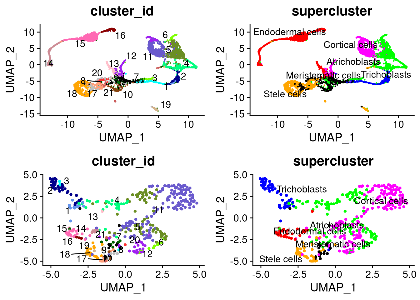
Figure 8.1: UMAP plots for Datasets 4 (bottom) and 5 (top)
We see that the data are not aligned across the two datasets.
8.4 Integrate the datasets
Now we are ready to integrate the two datasets. First we select a subset of features (genes) on which to base the integration.
my_datasets <- list(my_seurat_4, my_seurat_5) # you may have more than two datasets!
common_variable_features <- SelectIntegrationFeatures(my_datasets) # nfeatures = 2000 by default
We may inspect the selected genes,
head(common_variable_features)## [1] "AT4G15290" "AT5G37690" "AT5G42180" "AT2G36100" "AT1G53830" "AT2G23540"length(common_variable_features)## [1] 2000Next, we use the selected genes as input to FindIntegrationAnchors()
mutual_nearest_neighbors <- FindIntegrationAnchors(my_datasets, anchor.features = common_variable_features) # reduction = "cca" by default## Scaling features for provided objects## Finding all pairwise anchors## Running CCA## Merging objects## Finding neighborhoods## Finding anchors## Found 1974 anchors## Filtering anchors## Retained 1049 anchorsThis returns a table of mutual nearest neighbors, each pair of which has a score.
mutual_nearest_neighbors## An AnchorSet object containing 2098 anchors between 2 Seurat objects
## This can be used as input to IntegrateData.head(mutual_nearest_neighbors@anchors)## cell1 cell2 score dataset1 dataset2
## 1 2 3001 0.1470588 1 2
## 2 2 4443 0.3529412 1 2
## 3 2 4896 0.1764706 1 2
## 4 2 4026 0.1176471 1 2
## 5 2 4519 0.2941176 1 2
## 6 4 4969 0.7058824 1 2Finally, we integrate the datasets and return the result in my_integrated_dataset.
my_integrated_dataset <- IntegrateData(mutual_nearest_neighbors)## Merging dataset 1 into 2## Extracting anchors for merged samples## Finding integration vectors## Finding integration vector weights## Integrating data## Warning: Layer counts isn't present in the assay object; returning NULLmy_integrated_dataset## An object of class Seurat
## 25961 features across 5584 samples within 2 assays
## Active assay: integrated (2000 features, 2000 variable features)
## 1 layer present: data
## 1 other assay present: RNAInspect the integrated dataset’s assays,
my_integrated_dataset@assays## $RNA
## Assay (v5) data with 23961 features for 5584 cells
## Top 10 variable features:
## AT4G33790, AT1G03920, AT1G43020, AT3G54530, AT2G04050, AT4G15290,
## AT2G24850, AT3G51740, AT3G54520, AT4G33260
## Layers:
## counts.Dataset 4, counts.Dataset 5, data.Dataset 4, scale.data.Dataset
## 4, data.Dataset 5, scale.data.Dataset 5
##
## $integrated
## Assay data with 2000 features for 5584 cells
## Top 10 variable features:
## AT4G15290, AT5G37690, AT5G42180, AT2G36100, AT1G53830, AT2G23540,
## AT4G20390, AT1G54970, AT3G49960, AT2G24850Note that there are two assays, ‘integrated’ (the current default) and ‘RNA’ (the original assay, with unmodified data). Again, the integrated dataset is based on the top 2000 common variable features.
We may now run the usual analysis on the integrated dataset.
# DefaultAssay(my_integrated_dataset) <- "integrated"
my_integrated_dataset <- ScaleData(my_integrated_dataset, verbose = FALSE)
my_integrated_dataset <- RunPCA(my_integrated_dataset, verbose = FALSE)
set.seed(42)
my_integrated_dataset <- RunUMAP(my_integrated_dataset, dims = 1:20, verbose = FALSE)
# Put the factor levels in the correct order
my_integrated_dataset$cluster_id <- factor(my_integrated_dataset$cluster_id, levels = levels(my_seurat_5$cluster_id))
my_integrated_dataset$supercluster <- factor(my_integrated_dataset$supercluster, levels = levels(my_seurat_5$supercluster))

# Save the dataset if desired
# saveRDS(my_integrated_dataset, "data/my_integrated.rds")
We can see that the two datasets are now integrated,
pdf("pdf/integrated-dataset.pdf")
DimPlot(my_integrated_dataset)
dev.off()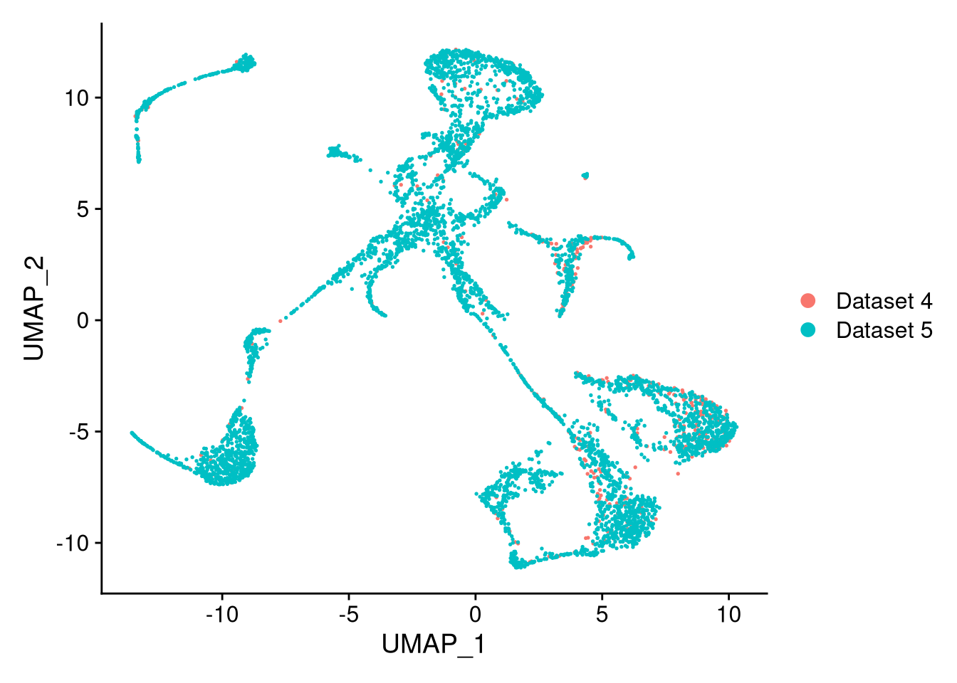
Figure 8.2: The integrated dataset
pdf("pdf/integrated-dataset-clusters.pdf")
DimPlot(my_integrated_dataset, cols = cluster_colors, group.by = "cluster_id", label.size = 4, repel = TRUE, label = TRUE)
dev.off()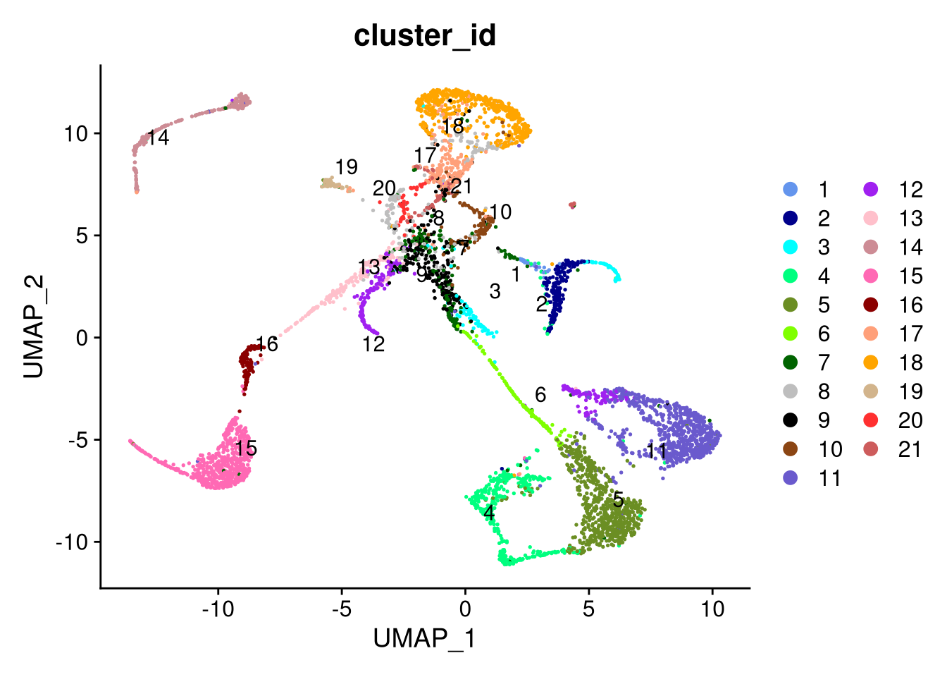
Figure 8.3: The integrated dataset, by cluster id
pdf("pdf/integrated-dataset-superclusters.pdf")
DimPlot(my_integrated_dataset, cols = supercluster_colors, group.by = "supercluster", label.size = 4, repel = TRUE, label = TRUE) + NoLegend()
dev.off()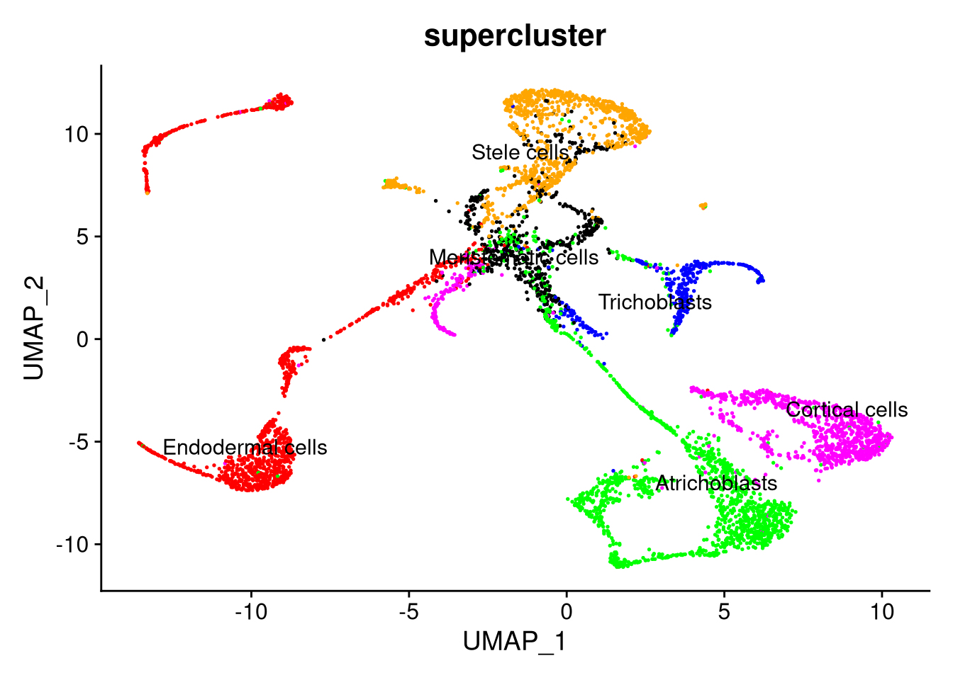
Figure 8.4: The integrated dataset, by supercluster
To compare the original datasets side by side after integration, use the split.by argument.
pdf("pdf/integrated-dataset-split.pdf")
DimPlot(my_integrated_dataset, split.by = "ident") + NoLegend()
dev.off()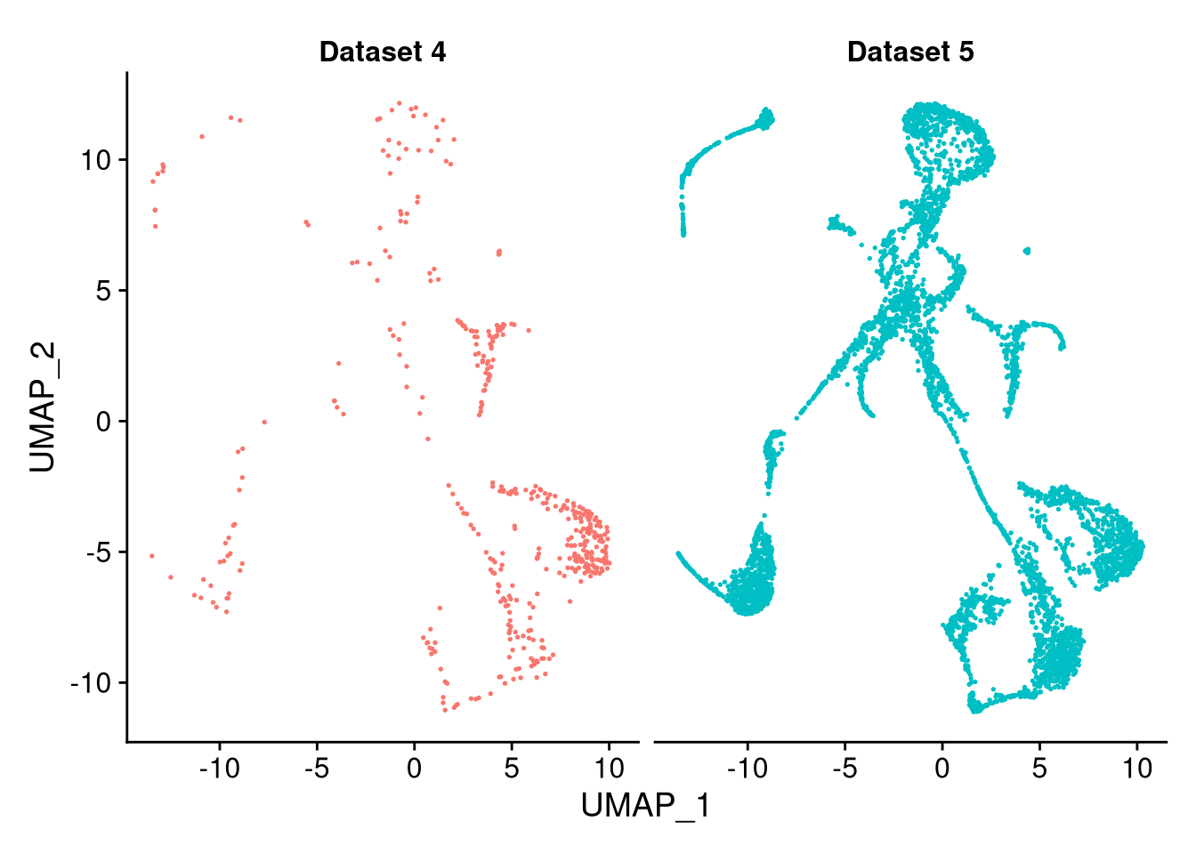
Figure 8.5: The integrated dataset, split by original dataset
8.5 Differential expression with integrated data
We can again look at differential expression through feature plots, dot plots, and violin plots. But now we may distinguish between the integrated datasets.
# JoinLayers() is required in Seurat v5, but not in Seurat v4 and earlier
my_integrated_dataset[["RNA"]] <- JoinLayers(my_integrated_dataset[["RNA"]])
DefaultAssay(my_integrated_dataset) <- "RNA"
my_markers <- FindAllMarkers(my_integrated_dataset, verbose = FALSE)
head(my_markers)
## p_val avg_log2FC pct.1 pct.2 p_val_adj cluster
## AT3G06355 1.586775e-200 -4.426622 0.353 0.980 3.802071e-196 Dataset 4
## AT1G73330 9.527465e-184 4.027308 0.982 0.682 2.282876e-179 Dataset 4
## AT2G01520 3.708981e-144 3.137345 0.968 0.531 8.887088e-140 Dataset 4
## AT1G20920 5.644810e-136 -2.760102 0.192 0.851 1.352553e-131 Dataset 4
## AT4G36648 5.595481e-129 -1.810522 0.693 0.980 1.340733e-124 Dataset 4
## AT1G73260 3.080499e-122 4.347956 0.515 0.130 7.381183e-118 Dataset 4
## gene
## AT3G06355 AT3G06355
## AT1G73330 AT1G73330
## AT2G01520 AT2G01520
## AT1G20920 AT1G20920
## AT4G36648 AT4G36648
## AT1G73260 AT1G73260# Retain top N genes for use in different plot types
top_8_genes <- head(my_markers$gene, 8)
top_4_genes <- head(my_markers$gene, 4)
top_2_genes <- head(my_markers$gene, 2)We can use a feature plot to split by dataset,
pdf("pdf/integration-featureplot.pdf")
FeaturePlot(my_integrated_dataset, features = top_2_genes, split.by = "orig.ident")
dev.off()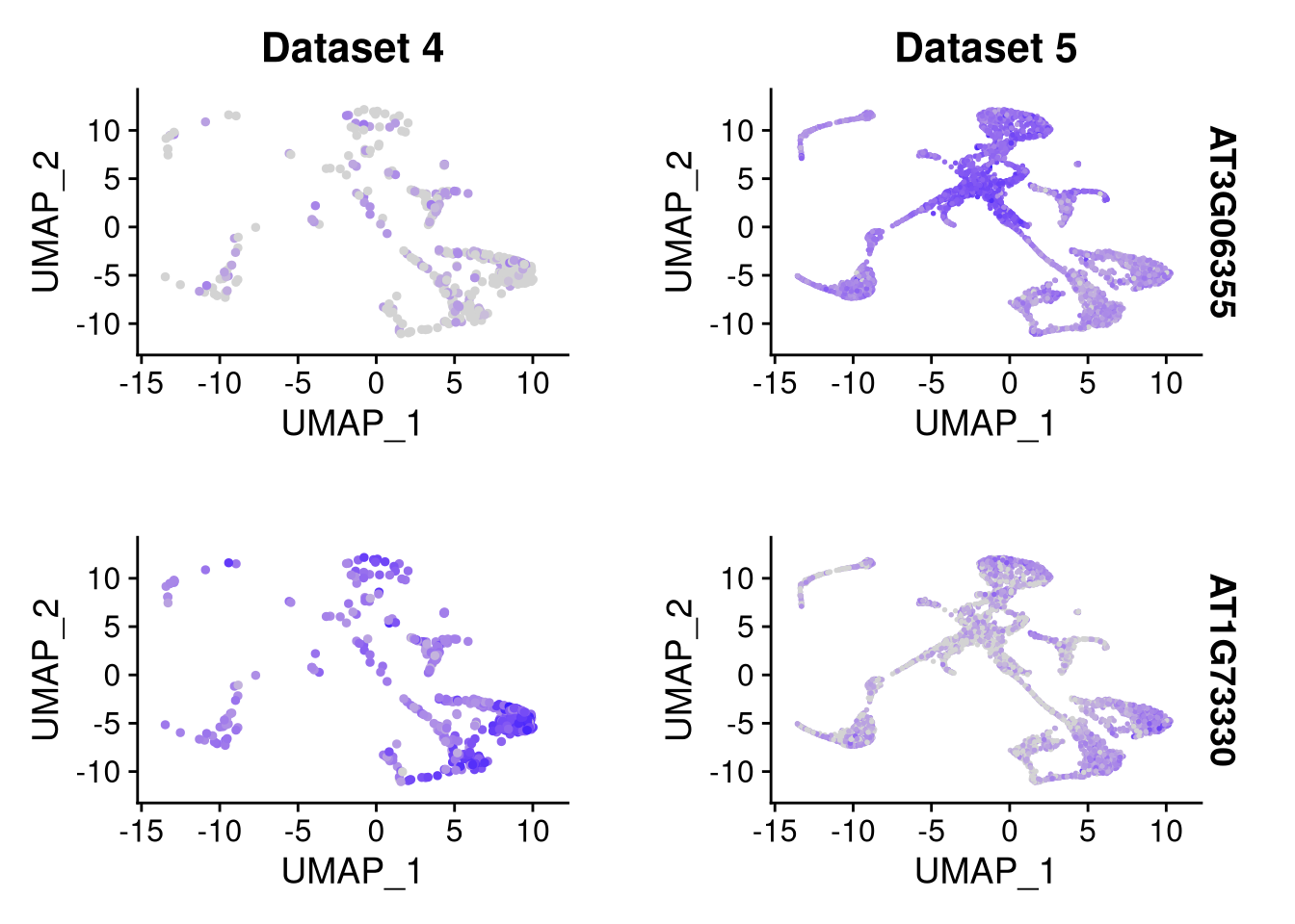
Figure 8.6: Feature plot for 2 datasets × 2 marker genes
We can also split dot plots by one or two identity variables (as they are two-dimensional). Here we just split by dataset,
pdf("pdf/integration-dotplot-dataset.pdf")
DotPlot(my_integrated_dataset, features = top_8_genes, cols = c("blue", "red"), dot.scale = 8) + RotatedAxis()
dev.off()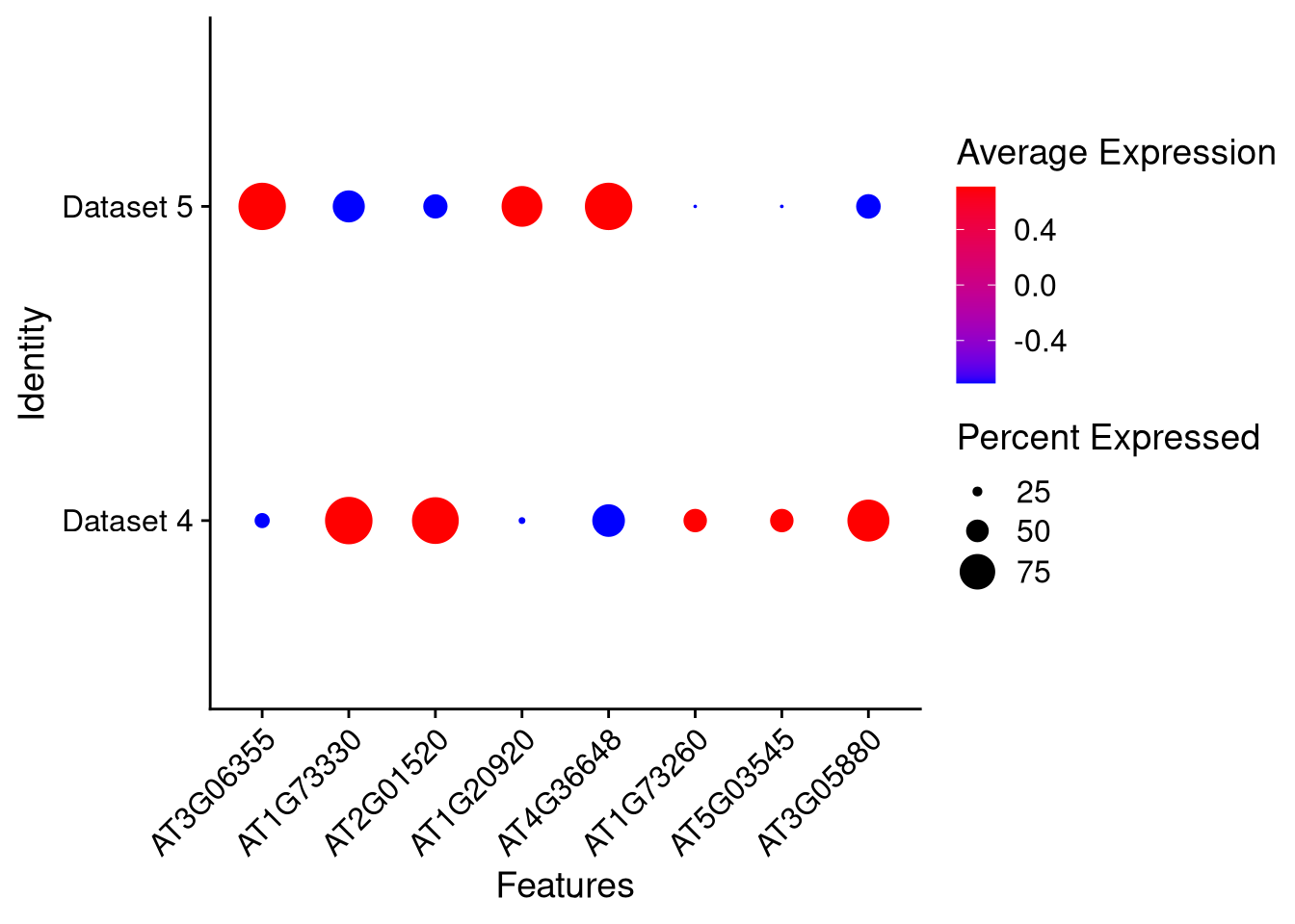
Figure 8.7: Dot plot for 8 marker genes, split by dataset
And here we split by supercluster as well. It splits and groups by orig.ident unless otherwise requested. For dot plots, the cols (colors) correspond to the split_by identity.
pdf("pdf/integration-dotplot-supercluster.pdf")
DotPlot(my_integrated_dataset, features = top_8_genes, cols = supercluster_colors, dot.scale = 8, split.by = "supercluster") + RotatedAxis()
dev.off()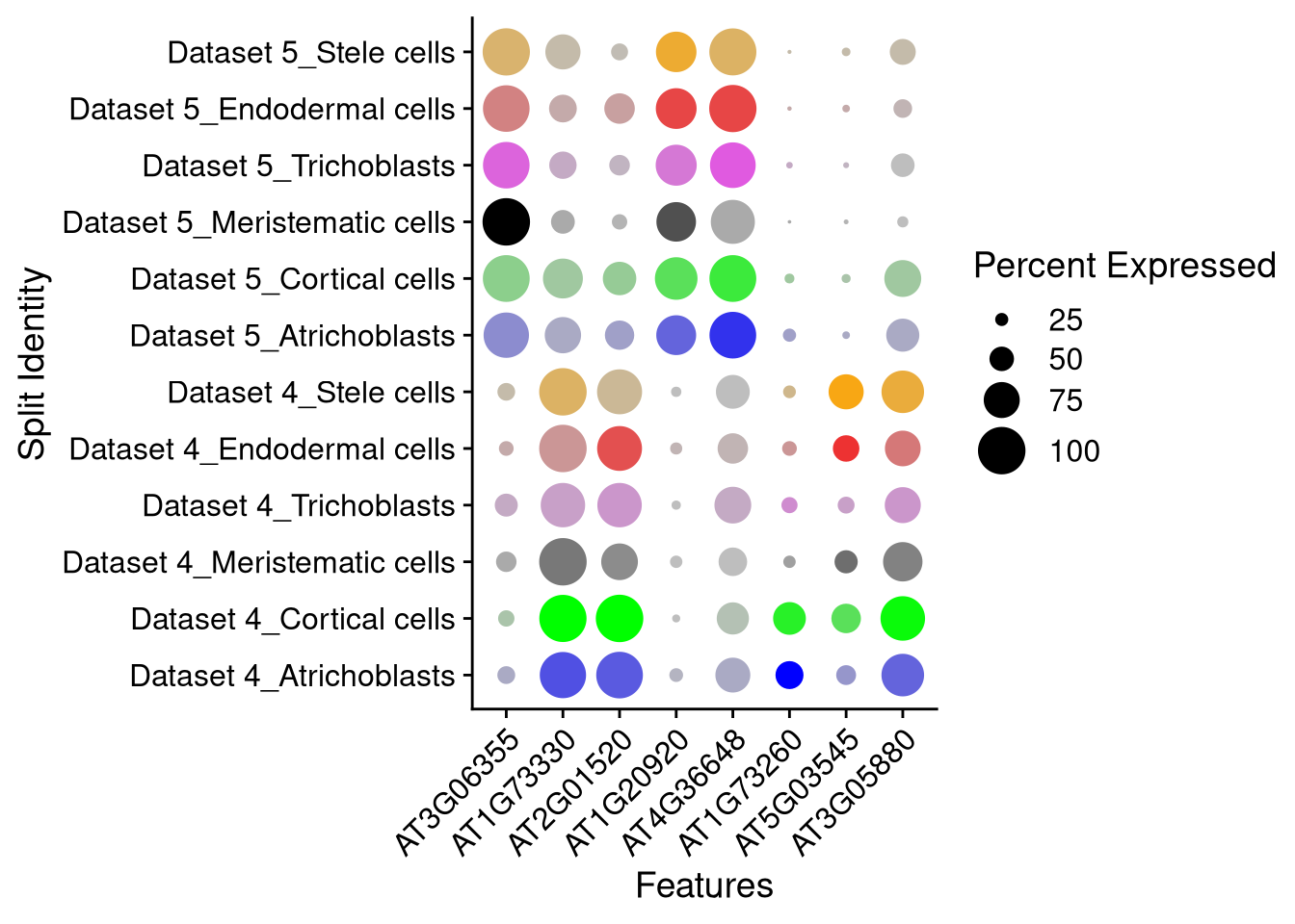
Figure 8.8: Dot plot for 8 marker genes, split by dataset and supercluster
We can do the same for violin plots, here just by dataset:
pdf("pdf/integration-violinplot-dataset.pdf")
plots <- VlnPlot(my_integrated_dataset, features = top_4_genes, pt.size = 0, combine = FALSE)
grid.arrange(plots[[1]], plots[[2]], plots[[3]], plots[[4]], ncol = 2)
dev.off()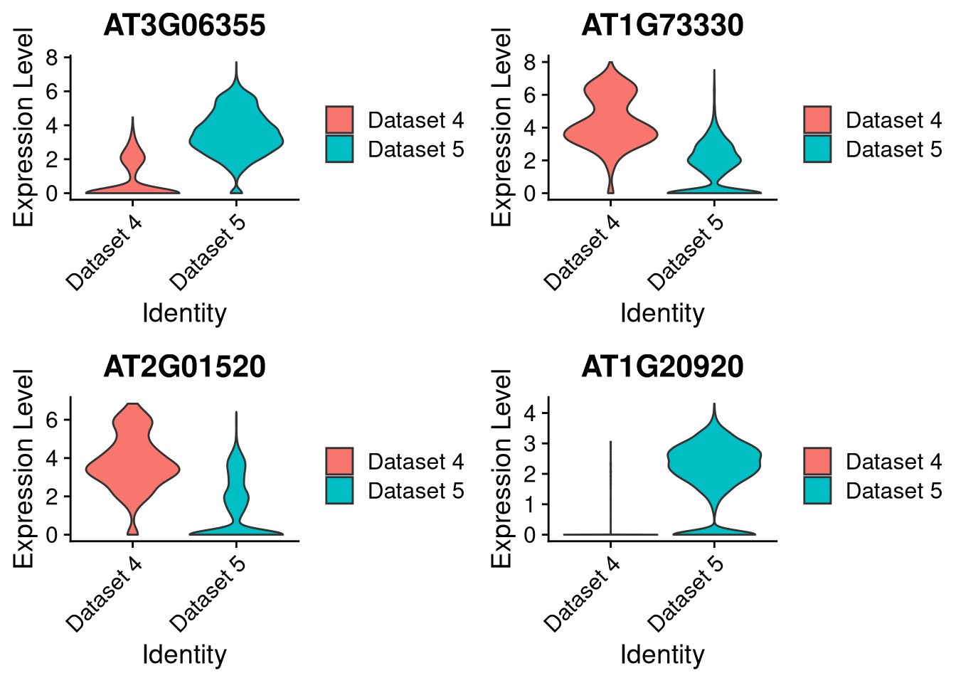
Figure 8.9: Violin plot for 4 marker genes, split by dataset
And here by dataset and supercluster. For violin plots, the legend and colors correspond to split.by, while the x axis categories correspond to group_by.
pdf("pdf/integration-violinplot-supercluster.pdf")
plots <- VlnPlot(my_integrated_dataset, features = top_4_genes, split.by = "orig.ident", group.by = "supercluster", pt.size = 0, combine = FALSE)
## The default behaviour of split.by has changed.
## Separate violin plots are now plotted side-by-side.
## To restore the old behaviour of a single split violin,
## set split.plot = TRUE.
##
## This message will be shown once per session.grid.arrange(plots[[1]], plots[[2]], plots[[3]], plots[[4]], ncol = 2)
dev.off()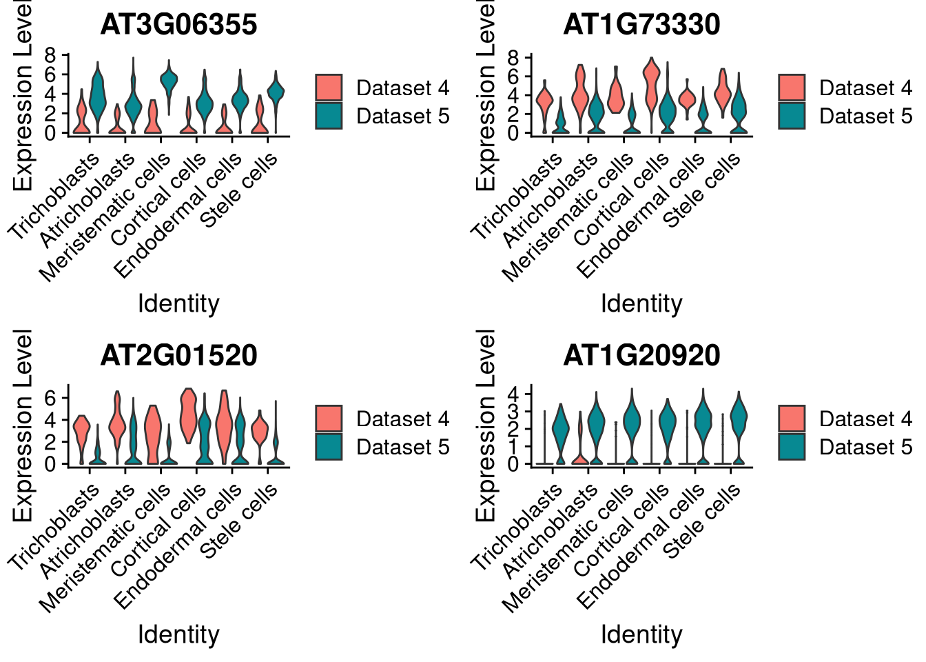
Figure 8.10: Violin plot for 4 marker genes, split by dataset and supercluster
You may also set split.plot = TRUE to produce split violins (heavy metal guitars?).
pdf("pdf/integration-splitviolinplot-supercluster.pdf")
plots <- VlnPlot(my_integrated_dataset, features = top_4_genes, split.by = "orig.ident", group.by = "supercluster", pt.size = 0, combine = FALSE, split.plot = TRUE)
grid.arrange(plots[[1]], plots[[2]], plots[[3]], plots[[4]], ncol = 2)
dev.off()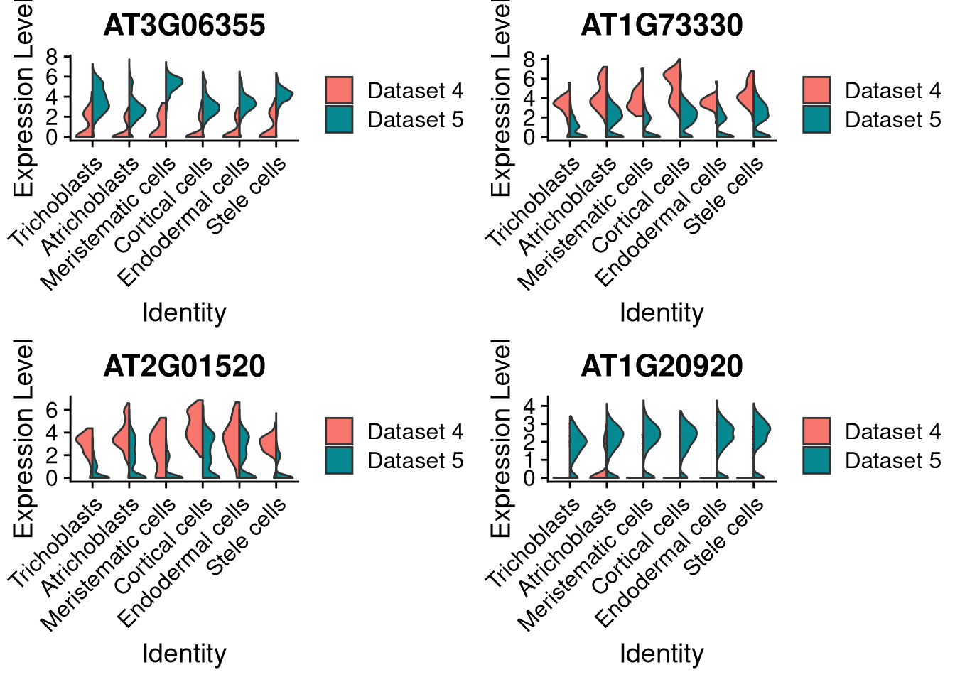
Figure 8.11: Same as above, with split violin plots
8.6 Further resources
Seurat - Data integration vignettes (from Vignettes menu)
Tran et al., A benchmark of batch-effect correction methods for single-cell RNA sequencing data, Genome Biology 21:12 (2020).