4 Bioconductor & SingleCellExperiment
Bioconductor is a collection of open source R packages for bioinformatics. These include several for single cell analysis, of which scater, scuttle, and SingleCellExperiment are of special interest.
Our required Bioconductor packages are already installed on the NCGR server. To install them on your own computer, you first need to install the BiocManager package from CRAN, then use BiocManager::install().
# No need to run this!
install.packages("BiocManager")
bioconductor_packages <- c("SingleCellExperiment", "scater") # and any others
BiocManager::install(bioconductor_packages)
4.1 SingleCellExperiment
The SingleCellExperiment class is the fundamental data structure of single cell analysis in Bioconductor. In this module, we will learn to create and import a SingleCellExperiment object, and extract its component parts. We begin by importing the required R packages.
library(SingleCellExperiment)
library(scater)
library(ggplot2)
library(gridExtra) # for multiple plots
4.2 Build a fake SCE from scratch
4.2.1 Generate counts
First we will create a small SingleCellExperiment from scratch, as a way to illustrate its components. We generate the count matrix from a exponential distribution rounded down to integers, just so the counts drop off rapidly from 0.
set.seed(42)
num_genes <- 12
num_cells <- 8
raw_counts <- as.integer(rexp(num_genes*num_cells, rate = 0.5))
raw_counts <- matrix(raw_counts, nrow = num_genes, ncol = num_cells)
4.2.2 Generate metadata
Now we can generate some metadata. For the rows, we give each gene a name and length, and for the columns we create a batch id and cell type in addition to its name.
gene_metadata <- data.frame(
  name = paste("Gene", 1:num_genes, sep = "_"),
  length = as.integer(rnorm(num_genes, mean = 10000, sd = 500))
)
cell_metadata <- data.frame(
  name = paste("Cell", 1:num_cells, sep = "_"),
  batch = rep(1:2, each = num_cells/2),
  tissue = rep(c("xylem", "phloem"), times = num_cells/2)
)
4.2.3 Create the SingleCellExperiment
And finally, we create the SingleCellExperiment object.
fake_SCE <- SingleCellExperiment(
  assays = list(counts = raw_counts), # wrap in a list
  rowData = gene_metadata,
  colData = cell_metadata,
  metadata = list(name = "Fake SCE")
)
fake_SCE
## class: SingleCellExperiment
## dim: 12 8
## metadata(1): name
## assays(1): counts
## rownames: NULL
## rowData names(2): name length
## colnames: NULL
## colData names(3): name batch tissue
## reducedDimNames(0):
## mainExpName: NULL
## altExpNames(0):4.2.4 Inspecting counts
The object summary listed above is quite terse, so let’s inspect its individual components. The assays() function lists the existing assays (the counts matrix and its transforms, which we will create below).
assays(fake_SCE)## List of length 1
## names(1): countsThere are three ways to access the counts matrix. Run each of them to confirm that they produce identical results.
# assays(fake_SCE)$counts
# assay(fake_SCE, "counts")
counts(fake_SCE)
## [,1] [,2] [,3] [,4] [,5] [,6] [,7] [,8]
## [1,] 0 0 2 0 0 0 1 2
## [2,] 1 0 1 0 13 2 1 0
## [3,] 0 2 2 0 0 0 2 0
## [4,] 0 0 0 3 3 0 13 0
## [5,] 0 0 0 1 2 0 2 0
## [6,] 2 1 2 1 0 0 0 1
## [7,] 0 2 1 0 1 3 1 5
## [8,] 0 0 6 2 0 1 2 3
## [9,] 2 9 0 3 2 0 2 4
## [10,] 1 1 0 0 1 0 0 2
## [11,] 2 9 3 8 0 11 0 1
## [12,] 4 0 1 2 16 0 0 3The syntax of the first two will work for any assay you define, but counts() is one of a handful of dedicated functions for commonly used assays. (We will discuss these in the Transform the raw counts section below.)
4.2.5 Inspecting metadata
We access row and column metadata through the rowData() and colData() functions.
rowData(fake_SCE)## DataFrame with 12 rows and 2 columns
## name length
## <character> <integer>
## 1 Gene_1 10797
## 2 Gene_2 9479
## 3 Gene_3 9771
## 4 Gene_4 9866
## 5 Gene_5 10379
## ... ... ...
## 8 Gene_8 10063
## 9 Gene_9 9573
## 10 Gene_10 9541
## 11 Gene_11 9762
## 12 Gene_12 9553colData(fake_SCE)## DataFrame with 8 rows and 3 columns
## name batch tissue
## <character> <integer> <character>
## 1 Cell_1 1 xylem
## 2 Cell_2 1 phloem
## 3 Cell_3 1 xylem
## 4 Cell_4 1 phloem
## 5 Cell_5 2 xylem
## 6 Cell_6 2 phloem
## 7 Cell_7 2 xylem
## 8 Cell_8 2 phloem4.3 Transform the raw counts
The raw counts matrix is simple to understand, but is often inefficient to analyze or visualize because the distribution of counts is skewed toward smaller values (in real experiments, most counts are zero). It is therefore advantageous to transform the counts, to effectively enhance the contrast between counts at the low end and make the overall distribution of transformed counts more symmetric (and closer to a normal distribution).
Here we will create some transformed count matrices by hand. Besides counts(), standard functions for SingleCellExperiment assays include normcounts(), logcounts(), and cpm().
4.3.1 Normalized counts
First, normcounts are normalized counts. The idea is that single cell count measurements may have systematic biases, for example variation in PCR amplification across experiments would cause the appearance of higher or lower counts. We can scale (or “normalize”) the counts to reduce such experimental bias, so that the differences in the cell counts more closely reflect the underlying biology.
There are many normalization methods (and schools of thought on the best way to normalize), but a simple way is to scale each cell’s counts by the total counts for the corresponding cell.
total_cell_counts <- colSums(counts(fake_SCE))
size_factor <- total_cell_counts/mean(total_cell_counts)
# t() ("transpose") flips the matrix rows and columns, so we have the right dimensions for the normalization
normcounts(fake_SCE) <- t(t(counts(fake_SCE))/size_factor)
normcounts(fake_SCE)
## [,1] [,2] [,3] [,4] [,5] [,6] [,7] [,8]
## [1,] 0.0000 0.00000 2.416667 0.0000 0.0000000 0.000000 0.90625 2.071429
## [2,] 1.8125 0.00000 1.208333 0.0000 7.4407895 2.558824 0.90625 0.000000
## [3,] 0.0000 1.81250 2.416667 0.0000 0.0000000 0.000000 1.81250 0.000000
## [4,] 0.0000 0.00000 0.000000 3.2625 1.7171053 0.000000 11.78125 0.000000
## [5,] 0.0000 0.00000 0.000000 1.0875 1.1447368 0.000000 1.81250 0.000000
## [6,] 3.6250 0.90625 2.416667 1.0875 0.0000000 0.000000 0.00000 1.035714
## [7,] 0.0000 1.81250 1.208333 0.0000 0.5723684 3.838235 0.90625 5.178571
## [8,] 0.0000 0.00000 7.250000 2.1750 0.0000000 1.279412 1.81250 3.107143
## [9,] 3.6250 8.15625 0.000000 3.2625 1.1447368 0.000000 1.81250 4.142857
## [10,] 1.8125 0.90625 0.000000 0.0000 0.5723684 0.000000 0.00000 2.071429
## [11,] 3.6250 8.15625 3.625000 8.7000 0.0000000 14.073529 0.00000 1.035714
## [12,] 7.2500 0.00000 1.208333 2.1750 9.1578947 0.000000 0.00000 3.107143t() do in our manual normcounts calculation?
Click for answer
It flips the columns and rows again, to restore the original matrix dimensions.Click for answer
head(colSums(normcounts(fake_SCE)))## [1] 21.75 21.75 21.75 21.75 21.75 21.75mean(colSums(counts(fake_SCE)))## [1] 21.754.3.2 Counts per million
cpm is counts per million, effectively normcounts with a different scale.
cpm(fake_SCE) <- 1000000*t(t(counts(fake_SCE))/total_cell_counts)
cpm(fake_SCE)
## [,1] [,2] [,3] [,4] [,5] [,6] [,7]
## [1,] 0.00 0.00 111111.11 0 0.00 0.00 41666.67
## [2,] 83333.33 0.00 55555.56 0 342105.26 117647.06 41666.67
## [3,] 0.00 83333.33 111111.11 0 0.00 0.00 83333.33
## [4,] 0.00 0.00 0.00 150000 78947.37 0.00 541666.67
## [5,] 0.00 0.00 0.00 50000 52631.58 0.00 83333.33
## [6,] 166666.67 41666.67 111111.11 50000 0.00 0.00 0.00
## [7,] 0.00 83333.33 55555.56 0 26315.79 176470.59 41666.67
## [8,] 0.00 0.00 333333.33 100000 0.00 58823.53 83333.33
## [9,] 166666.67 375000.00 0.00 150000 52631.58 0.00 83333.33
## [10,] 83333.33 41666.67 0.00 0 26315.79 0.00 0.00
## [11,] 166666.67 375000.00 166666.67 400000 0.00 647058.82 0.00
## [12,] 333333.33 0.00 55555.56 100000 421052.63 0.00 0.00
## [,8]
## [1,] 95238.10
## [2,] 0.00
## [3,] 0.00
## [4,] 0.00
## [5,] 0.00
## [6,] 47619.05
## [7,] 238095.24
## [8,] 142857.14
## [9,] 190476.19
## [10,] 95238.10
## [11,] 47619.05
## [12,] 142857.14Again confirm the normalization,
colSums(cpm(fake_SCE))## [1] 1e+06 1e+06 1e+06 1e+06 1e+06 1e+06 1e+06 1e+06As expected, the “total cell count” for counts per million is 1 million for each cell.
4.3.3 Log-normalized counts
Normalization alone does not achieve our goal of unskewing the distribution of counts. The simplest way is to take the logarithm of the normalized counts (adding 1 so that the values for zero counts remain zero), resulting in the log-normalized counts.
logcounts(fake_SCE) <- log2(normcounts(fake_SCE) + 1)
logcounts(fake_SCE)
## [,1] [,2] [,3] [,4] [,5] [,6] [,7]
## [1,] 0.000000 0.0000000 1.772590 0.000000 0.0000000 0.000000 0.9307373
## [2,] 1.491853 0.0000000 1.142958 0.000000 3.0773779 1.831400 0.9307373
## [3,] 0.000000 1.4918531 1.772590 0.000000 0.0000000 0.000000 1.4918531
## [4,] 0.000000 0.0000000 0.000000 2.091700 1.4420705 0.000000 3.6759570
## [5,] 0.000000 0.0000000 0.000000 1.061776 1.1008006 0.000000 1.4918531
## [6,] 2.209453 0.9307373 1.772590 1.061776 0.0000000 0.000000 0.0000000
## [7,] 0.000000 1.4918531 1.142958 0.000000 0.6529393 2.274481 0.9307373
## [8,] 0.000000 0.0000000 3.044394 1.666757 0.0000000 1.188662 1.4918531
## [9,] 2.209453 3.1947569 0.000000 2.091700 1.1008006 0.000000 1.4918531
## [10,] 1.491853 0.9307373 0.000000 0.000000 0.6529393 0.000000 0.0000000
## [11,] 2.209453 3.1947569 2.209453 3.277985 0.0000000 3.913945 0.0000000
## [12,] 3.044394 0.0000000 1.142958 1.666757 3.3445295 0.000000 0.0000000
## [,8]
## [1,] 1.618910
## [2,] 0.000000
## [3,] 0.000000
## [4,] 0.000000
## [5,] 0.000000
## [6,] 1.025535
## [7,] 2.627273
## [8,] 2.038135
## [9,] 2.362570
## [10,] 1.618910
## [11,] 1.025535
## [12,] 2.038135Note that logcounts is the default assay for many of the charting functions, so if you do not compute it, you will have to override that argument (exprs_values = ...) to the chart. (We will see examples in the Dimensionality Reduction chapter.)
Inspecting our assays shows that four counts matrices are now present.
assays(fake_SCE)## List of length 4
## names(4): counts normcounts cpm logcountsBefore we move on to real data, note that creating simulated single cell data (for example, in order to test your analysis pipeline before collecting data) need not be as labor-intensive as we made it for fake_SCE. The scuttle package has a mockSCE() function that does much of the work.
4.4 Create a SingleCellExperiment by importing data
Now that we know our way around the SingleCellExperiment object, we will import single cell nucleus RNA-seq data from Farmer et al. (2021). This study identified cell subtypes by their differential accessibility of chromatin (which regulates gene expression) in root cells in the model plant Arabidopsis thaliana. Our goal is to reproduce (some of) their results, using a subset of their data (one of five samples).
As the data files we will use are buried deep in a data subdirectory on the NCGR server, it is a good idea to create an easily accessible symbolic link to their location. You have already seen the ln -s command in the Linux module, now we will use it to create a symbolic link called ‘data’. Rather than quitting R and running the command from Linux, which would lose all the work we have done so far, we can run a Linux command from within R using the system() function. (This works on Macintosh or Windows operating systems as well, though their commands would be different.)
if (!file.exists("data")) system("ln -s /home/data/single-cell-workshop/data-farmer-et-al/sNucRNA-seq_rep5/ data")Click for answer
list.files("data")Now, import the data into a SingleCellExperiment called my_SCE.
my_SCE <- DropletUtils::read10xCounts("data/filtered_feature_bc_matrix/", col.names = TRUE, compressed = TRUE)Note that counts(my_SCE) is a sparse matrix. As most of the elements are zero, it stores only nonzero counts in order to save memory.
counts(my_SCE)[1:6, 1:3]## 6 x 3 sparse Matrix of class "dgCMatrix"
## AAACCCACACGCGCAT-1 AAACCCACAGAAGTTA-1 AAACCCACAGACAAAT-1
## AT1G01010 . 1 .
## AT1G01020 . . 1
## AT1G03987 . . .
## AT1G01030 . . .
## AT1G01040 . . 2
## AT1G03993 . . .dim(my_SCE)## [1] 34218 5780Click for answer
See the result ofdim(my_SCE): 34218 genes × 5780 cells.
head(rowData(my_SCE))## DataFrame with 6 rows and 3 columns
## ID Symbol Type
## <character> <character> <character>
## AT1G01010 AT1G01010 AT1G01010 Gene Expression
## AT1G01020 AT1G01020 AT1G01020 Gene Expression
## AT1G03987 AT1G03987 AT1G03987 Gene Expression
## AT1G01030 AT1G01030 AT1G01030 Gene Expression
## AT1G01040 AT1G01040 AT1G01040 Gene Expression
## AT1G03993 AT1G03993 AT1G03993 Gene Expressionhead(colData(my_SCE))## DataFrame with 6 rows and 2 columns
## Sample Barcode
## <character> <character>
## AAACCCACACGCGCAT-1 data/filtered_featur.. AAACCCACACGCGCAT-1
## AAACCCACAGAAGTTA-1 data/filtered_featur.. AAACCCACAGAAGTTA-1
## AAACCCACAGACAAAT-1 data/filtered_featur.. AAACCCACAGACAAAT-1
## AAACCCACATTGACAC-1 data/filtered_featur.. AAACCCACATTGACAC-1
## AAACCCAGTAGCTTTG-1 data/filtered_featur.. AAACCCAGTAGCTTTG-1
## AAACCCAGTCCAGTTA-1 data/filtered_featur.. AAACCCAGTCCAGTTA-1Click for answer
Row metadata: ID and Symbol are the gene id, Type is “Gene Expression”.
Sample is the name of the subdirectory from which we read the data, Barcode is the cell barcode. So these are very basic metadata so far.
ID and Symbol appear identical. Are they?
Click for answer
all(rowData(my_SCE)$ID == rowData(my_SCE)$Symbol)## [1] TRUEType values identical? What about the column metadata Sample values?
Click for answer
all(rowData(my_SCE)$Type == rowData(my_SCE)$Type[1])## [1] TRUEall(colData(my_SCE)$Sample == colData(my_SCE)$Sample[1])## [1] TRUE# or alternatively,
length(unique(rowData(my_SCE)$Type)) == 1## [1] TRUElength(unique(colData(my_SCE)$Sample)) == 1## [1] TRUE4.5 Predefined count transformations
In our fake_SCE example, we computed the log-normalized counts and other transformed count matrices by hand. However, functions from the scuttle package like logNormCounts(), normalizeCounts(), and calculateCPM() can do this for you, with the advantage that they keep the matrices sparse.
my_SCE <- logNormCounts(my_SCE)
# which is equivalent to
# assay(my_SCE, "logcounts") <- normalizeCounts(my_SCE) # log = TRUE by default
head(colData(my_SCE))
## DataFrame with 6 rows and 3 columns
## Sample Barcode sizeFactor
## <character> <character> <numeric>
## AAACCCACACGCGCAT-1 data/filtered_featur.. AAACCCACACGCGCAT-1 0.764455
## AAACCCACAGAAGTTA-1 data/filtered_featur.. AAACCCACAGAAGTTA-1 0.872851
## AAACCCACAGACAAAT-1 data/filtered_featur.. AAACCCACAGACAAAT-1 1.576417
## AAACCCACATTGACAC-1 data/filtered_featur.. AAACCCACATTGACAC-1 2.051818
## AAACCCAGTAGCTTTG-1 data/filtered_featur.. AAACCCAGTAGCTTTG-1 0.415850
## AAACCCAGTCCAGTTA-1 data/filtered_featur.. AAACCCAGTCCAGTTA-1 0.366336assay(my_SCE, "normcounts") <- normalizeCounts(my_SCE, log = FALSE)
assay(my_SCE, "cpm") <- calculateCPM(my_SCE)
counts(my_SCE)[1:6, 1:3]## 6 x 3 sparse Matrix of class "dgCMatrix"
## AAACCCACACGCGCAT-1 AAACCCACAGAAGTTA-1 AAACCCACAGACAAAT-1
## AT1G01010 . 1 .
## AT1G01020 . . 1
## AT1G03987 . . .
## AT1G01030 . . .
## AT1G01040 . . 2
## AT1G03993 . . .normcounts(my_SCE)[1:6, 1:3]## 6 x 3 sparse Matrix of class "dgCMatrix"
## AAACCCACACGCGCAT-1 AAACCCACAGAAGTTA-1 AAACCCACAGACAAAT-1
## AT1G01010 . 1.145671 .
## AT1G01020 . . 0.6343498
## AT1G03987 . . .
## AT1G01030 . . .
## AT1G01040 . . 1.2686995
## AT1G03993 . . .cpm(my_SCE)[1:6, 1:3]## 6 x 3 sparse Matrix of class "dgCMatrix"
## AAACCCACACGCGCAT-1 AAACCCACAGAAGTTA-1 AAACCCACAGACAAAT-1
## AT1G01010 . 383.2886 .
## AT1G01020 . . 212.2241
## AT1G03987 . . .
## AT1G01030 . . .
## AT1G01040 . . 424.4482
## AT1G03993 . . .logcounts(my_SCE)[1:6, 1:3]## 6 x 3 sparse Matrix of class "dgCMatrix"
## AAACCCACACGCGCAT-1 AAACCCACAGAAGTTA-1 AAACCCACAGACAAAT-1
## AT1G01010 . 1.101429 .
## AT1G01020 . . 0.7087168
## AT1G03987 . . .
## AT1G01030 . . .
## AT1G01040 . . 1.1818655
## AT1G03993 . . .Also note that logNormCounts() creates a new column of metadata, sizeFactor which is the scaling factor for normalized cell counts.
We can make histograms to confirm that the distribution of log-normalized counts is unskewed from that of the raw counts. (Note that for a sparse matrix of type dgCMatrix, the @x notation gives us a vector of its nonzero values.)
pdf("pdf/unskewing.pdf")
plot1 <- ggplot(mapping = aes(x = counts(my_SCE)@x)) +
  geom_histogram(fill = "#FF8000", bins = 100) +
  xlab("counts(my_SCE)") +
  xlim(0, 20)
plot2 <- ggplot(mapping = aes(x = logcounts(my_SCE)@x)) +
  geom_histogram(fill = "#0080FF", bins = 100) +
  xlab("logcounts(my_SCE)") +
  xlim(0, 3)
grid.arrange(plot1, plot2, ncol = 2)
dev.off()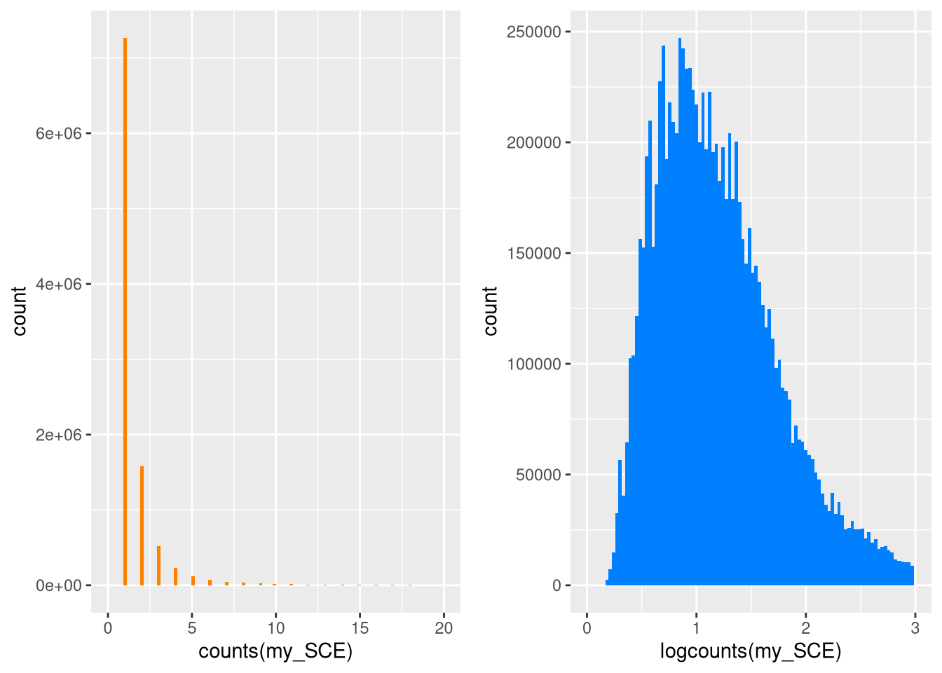
Figure 4.1: Distribution of raw and log-normalized counts
4.6 Statistical metrics
Let’s practice computing statistical metrics on genes and cells. We have already used colSums() to find the total counts for each cell,
total_cell_counts <- colSums(counts(my_SCE))
head(total_cell_counts)
## AAACCCACACGCGCAT-1 AAACCCACAGAAGTTA-1 AAACCCACAGACAAAT-1 AAACCCACATTGACAC-1
## 2285 2609 4712 6133
## AAACCCAGTAGCTTTG-1 AAACCCAGTCCAGTTA-1
## 1243 1095Click for answer
top_cells_by_counts <- sort(total_cell_counts, decreasing = TRUE)
head(top_cells_by_counts)
## GTAGATCGTGCACGCT-1 TCAGTGAAGGGCAGTT-1 AAGCCATAGTCATGCT-1 CTGCGAGGTTGCTCAA-1
## 21195 19958 18559 18471
## AGACCATAGCCGGATA-1 GCTCAAAAGGAAACGA-1
## 17360 16978top_100_cells <- names(top_cells_by_counts[1:100])Click for answer
total_gene_counts <- rowSums(counts(my_SCE))
head(sort(total_gene_counts, decreasing = TRUE))
## AT3G09260 AT4G36648 AT3G06355 ATMG00020 AT4G23670 AT5G48010
## 159791 117047 116963 83405 58408 57321Click for answer
sum(total_gene_counts > 0)## [1] 24015sum(total_gene_counts == 0)## [1] 10203Click for answer
num_genes_expressed_per_cell <- colSums(counts(my_SCE) > 0)
head(sort(num_genes_expressed_per_cell, decreasing = TRUE))
## AGCATCACACCATATG-1 AGGTAGGAGAATGTTG-1 AGACCATAGCCGGATA-1 TGCGGGTGTATCTTCT-1
## 6563 6438 6207 6206
## AGCTTCCGTTGTTTGG-1 GACTTCCCACAATGTC-1
## 6089 6012Click for answer
num_cells_gene_expressed <- rowSums(counts(my_SCE) > 0)
head(sort(num_cells_gene_expressed, decreasing = TRUE))
## ATMG00020 AT3G06355 AT4G36648 AT3G09260 AT4G39260 AT4G32850
## 5759 5640 5598 5525 5282 5035top_6_genes <- names(head(sort(num_cells_gene_expressed, decreasing = TRUE)))4.7 Visualize the data
The scater package includes various charting functions based on ggplot() but adapted to single-cell data. We will examine a few of the more useful ones, beginning with plotExpression().
pdf("pdf/plotExpression.pdf")
plotExpression(my_SCE, features = top_6_genes)
dev.off()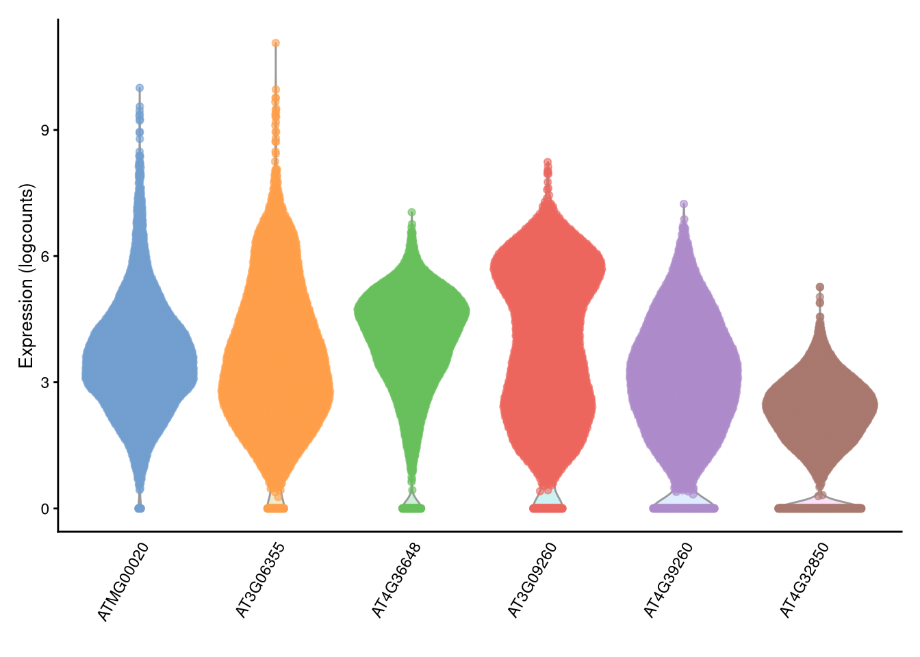
Figure 4.2: plotExpression() example
plotExpression() with counts instead of logcounts.
Click for answer
pdf("pdf/plotExpression-counts.pdf")
plotExpression(my_SCE, features = top_6_genes, exprs_values = "counts")
dev.off()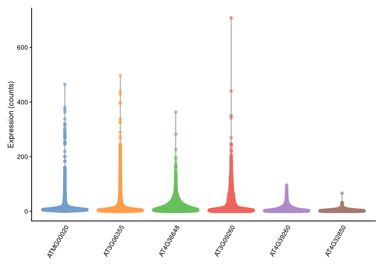
Figure 4.3: plotExpression() example with raw counts
The plotColData() function (in package scater) plots column metadata against each other. We will add our total_counts and num_genes_expressed_per_cell to the column metadata, and can plot them alone or against each other.
my_SCE$total_counts <- colSums(counts(my_SCE))
my_SCE$num_genes_expressed <- num_genes_expressed_per_cellpdf("pdf/plotColData-total-counts.pdf")
plotColData(my_SCE, "total_counts", "Sample", colour_by = "Sample") +
theme(legend.position = "none")
dev.off()
pdf("pdf/plotColData-num-genes-expressed.pdf")
plotColData(my_SCE, "num_genes_expressed", "Sample", colour_by = "Sample") +
theme(legend.position = "none")
dev.off()
# 2nd argument is y, 3rd is x (see ?plotColData for help)
pdf("pdf/plotColData-total-counts-x-num-genes-expressed.pdf")
plotColData(my_SCE, "num_genes_expressed", "total_counts", colour_by = "Sample") +
theme(legend.position = "none")
dev.off()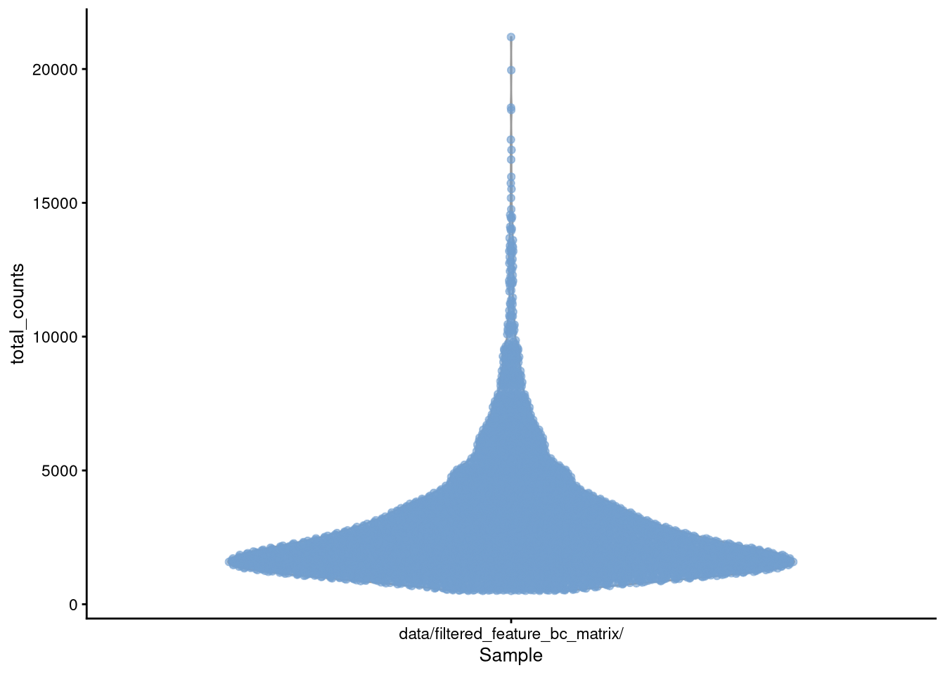
Figure 4.4: plotColData() for total_counts
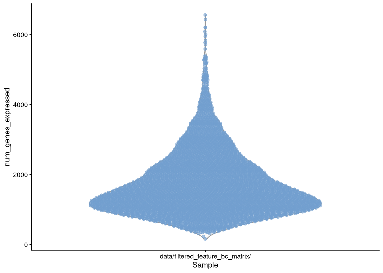
Figure 4.5: plotColData() for num_genes_expressed
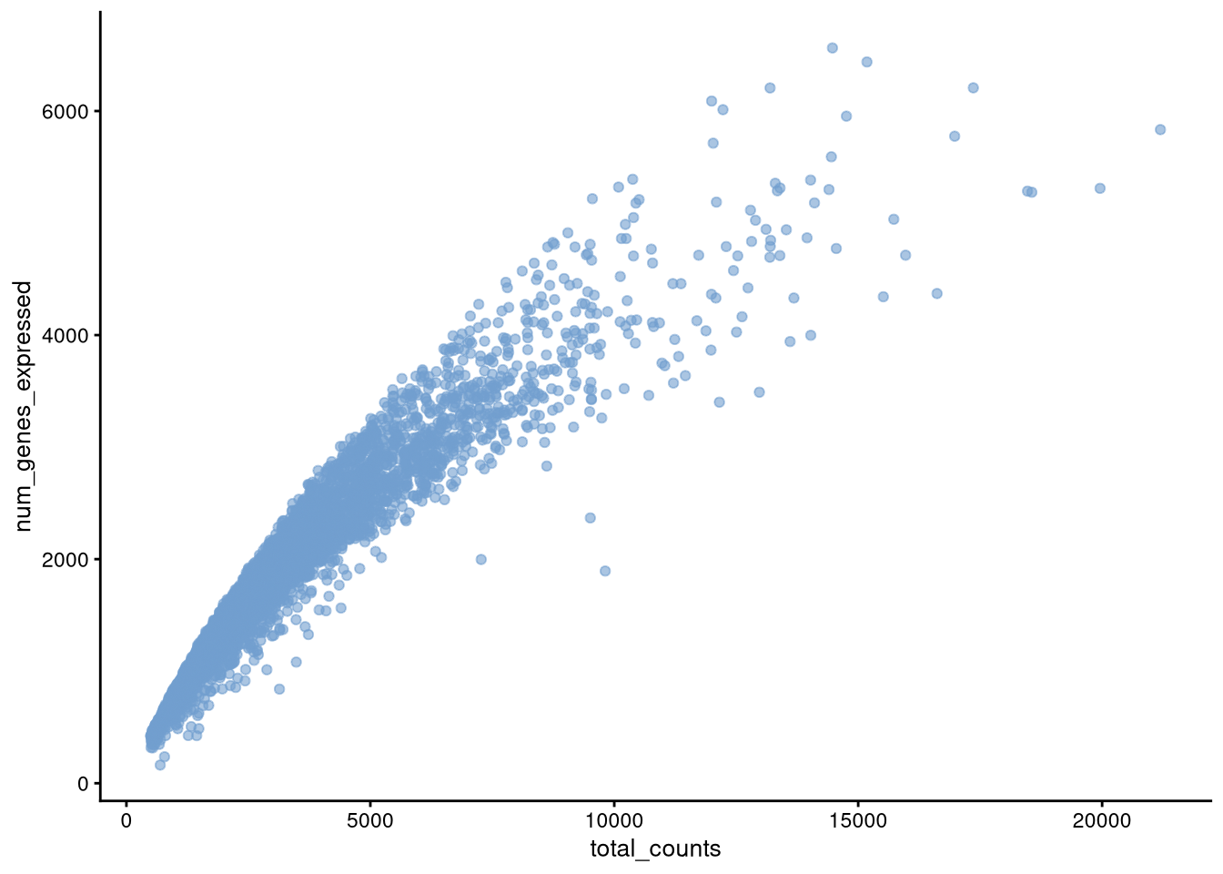
Figure 4.6: plotColData() for total_counts v. num_genes_expressed
When we use ggplot() directly, we normally pass it a single data frame, but in a SingleCellExperiment the relevant data may be divided across the assays, rowData, and colData. The ggcells() function (in package scater) automatically (and internally) combines SingleCellExperiment data into a single intermediate data frame, so that you need not worry about doing it manually.
As an example, we will create the same chart using both ggplot() and ggcells(). For ggcells(), note that the first argument is a SingleCellExperiment instead of a data frame, which simplifies the syntax.
pdf("pdf/ggcells.pdf")
plot1 <- ggplot(as.data.frame(colData(my_SCE)), aes(x = Sample, y = total_counts)) +
  geom_violin(fill = 'red') +
  ggtitle("ggplot()")
plot2 <- ggcells(my_SCE, aes(x = Sample, y = total_counts)) +
  geom_violin(fill = 'green') +
  ggtitle("ggcells()")
grid.arrange(plot1, plot2, ncol = 2)
dev.off()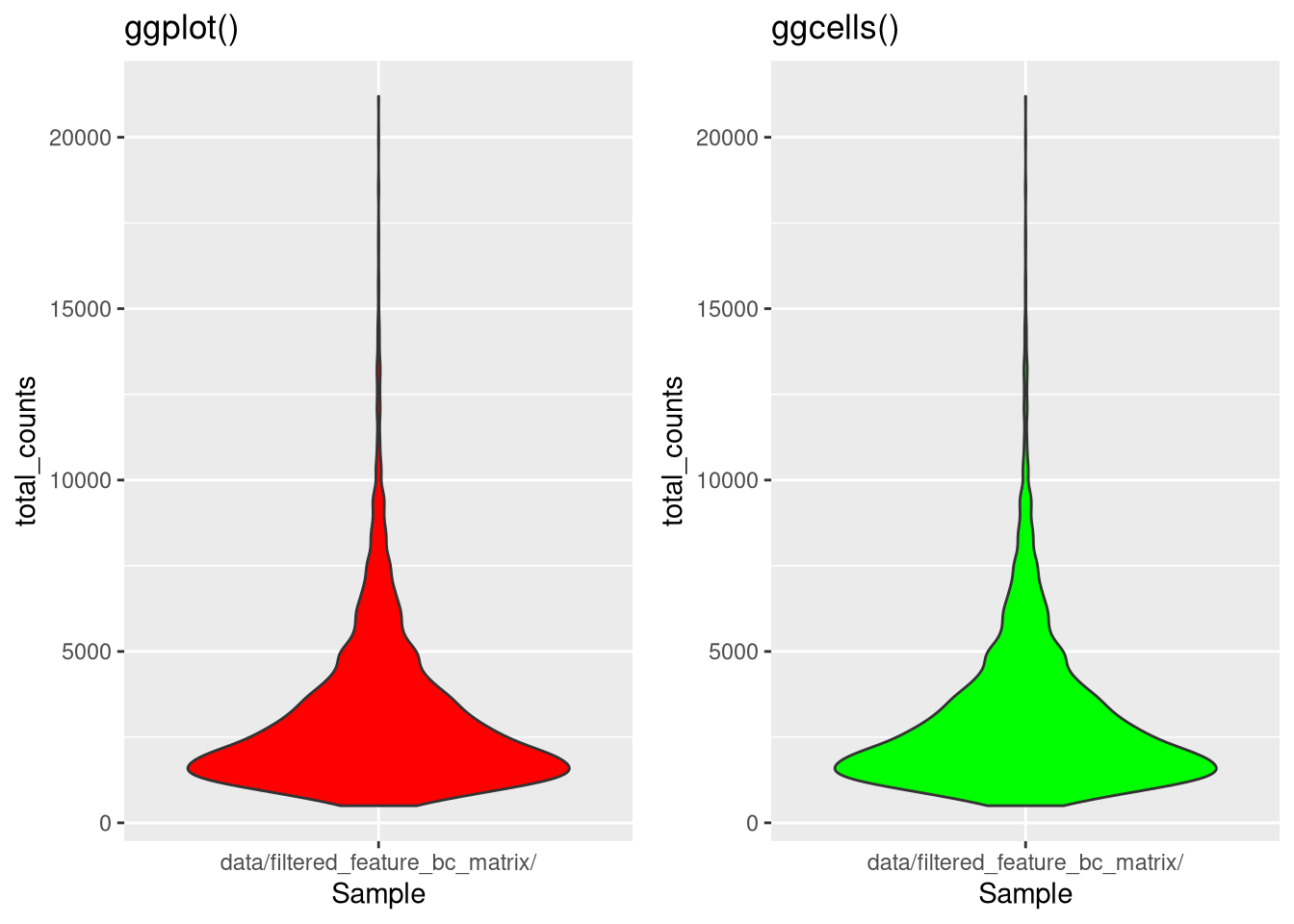
Figure 4.7: Same chart (different colors) with ggplot() and ggcells()
plotHighestExprs() is another way to show the distribution of cell counts for each gene. It takes a long time to build this chart for the whole data set, so here we consider only 25 genes and 100 cells.
pdf("pdf/plotHighestExprs.pdf")
plotHighestExprs(my_SCE[, top_100_cells], n = 25, exprs_values = "logcounts", colour_cells_by = "num_genes_expressed") # top n genes
dev.off()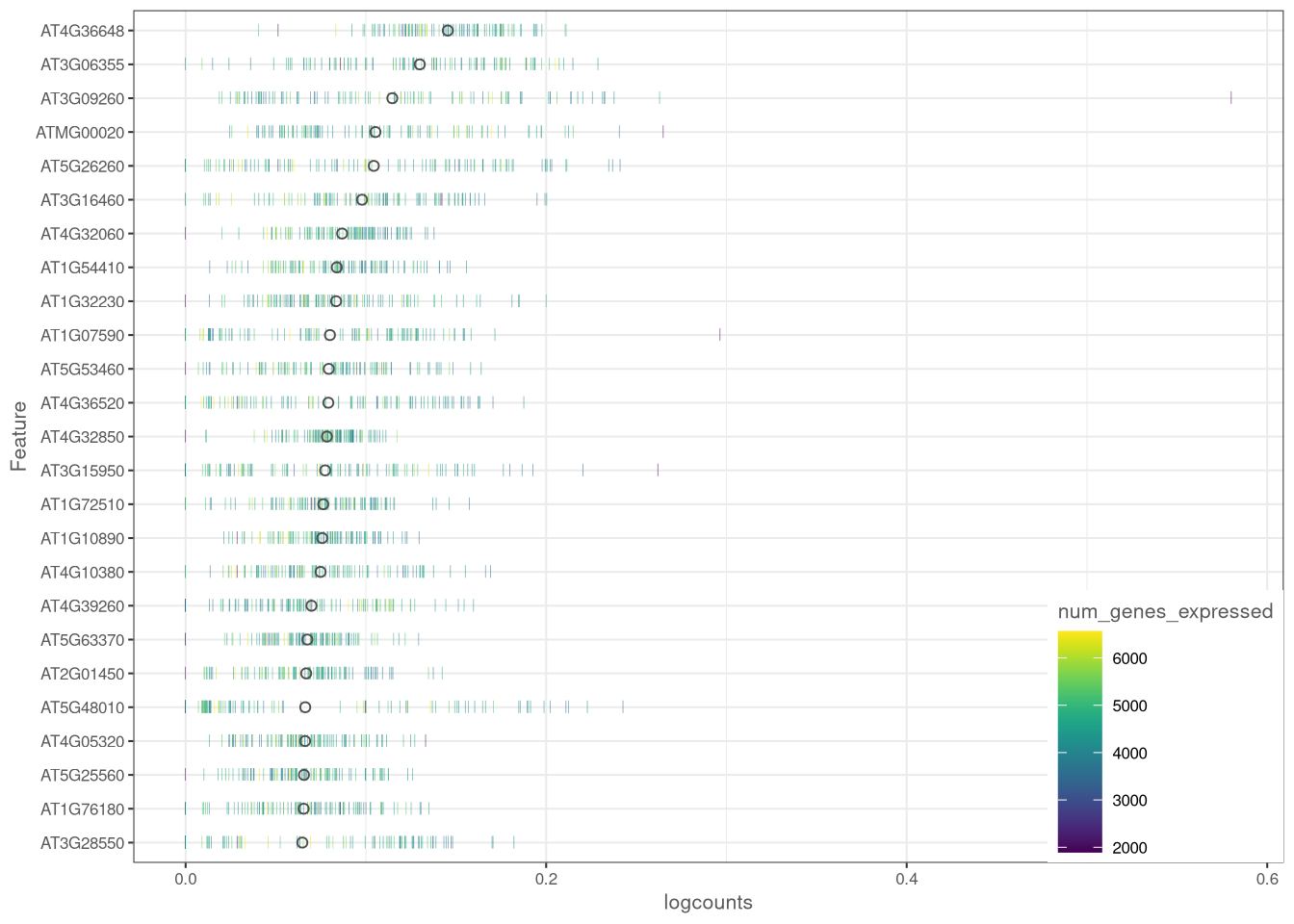
Figure 4.8: plotHighestExprs() example
plotHeatmap() automatically adds a dendrogram indicating clusters.
pdf("pdf/plotHeatmap.pdf")
plotHeatmap(my_SCE[, top_100_cells[1:6]], features = top_6_genes, show_colnames = TRUE)
dev.off()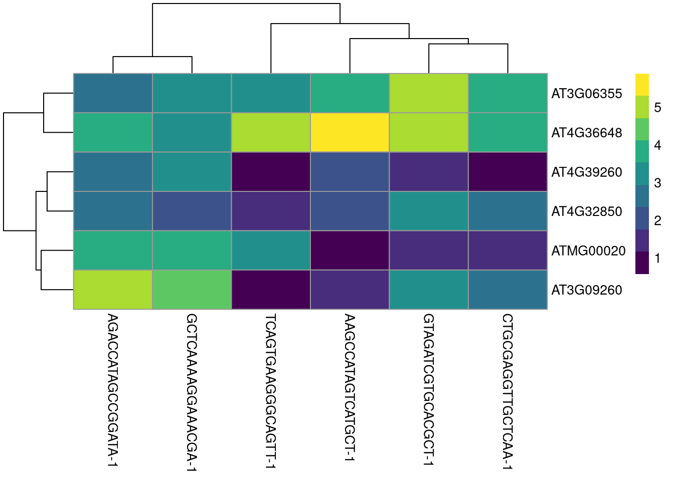
Figure 4.9: plotHeatmap() example
plotScater() shows how many genes are required to account for a given percentage of counts for each cell.
pdf("pdf/plotScater.pdf")
plotScater(my_SCE[, top_100_cells])
dev.off()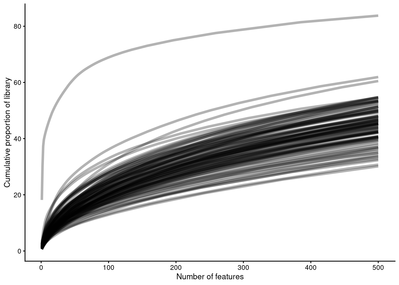
Figure 4.10: plotScater() example
Save the current SingleCellExperiment
Since we are at the end of the chapter, now would be a good time to save the current state of my_SCE. This would allow us to exit R, then begin the next chapter without rerunning this one. In general, it is wise to save such intermediate steps within your workflow.
# Do not run - depends on workshop timing
# saveRDS(my_SCE, "data/my_SCE-03.rds")
4.8 Further resources
4.8.1 Bioconductor packages and vignettes
Vignettes are concise tutorials that come with many R packages and all Bioconductor packages. You can access them through the package’s Bioconductor site, or from within R using the browseVignettes() function, which launches a web page with links to available vignette pages.
This does not work on the NCGR server (as no web browser is set up there), but you may try it on your own computer if you have R installed.
# for example,
# browseVignettes("SingleCellExperiment")Amezquita et al., Orchestrating single-cell analysis with Bioconductor, Nature Methods 17, 137–145 (2020).
McCarthy, Campbell, Lun, and Wills, Scater: pre-processing, quality control, normalization and visualization of single-cell RNA-seq data in R, Bioinformatics 33:8, 1179–1186 (2017).