2 Biological Context
Where does the sequening data come from? Once we have analysed our sequencing data, how does it translate back to cells, tissues, and organisms?
2.1 What is Single Cell RNA Seq (scRNA-seq)?
To understand what single cell RNA Seq is, we can compare and contrast with Bulk RNA Seq. Let’s walk through the bulk RNA Seq workflow below:
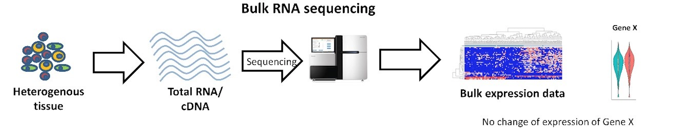
Bulk RNASeq
- An estimation of the average expression level for each gene within a population of cells
- Population-level resolution
- DNA from every cell in the sample is mixed together for sequencing
- Expression levels from every cell type are lumped together
Now let’s walk throug the Single Cell RNA Seq workflow:
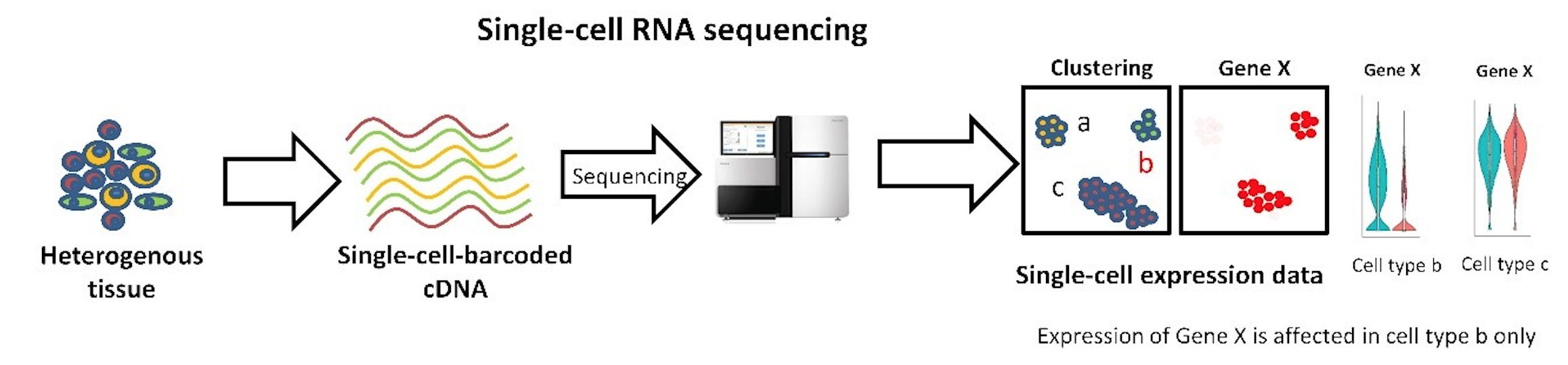
Single Cell RNASeq
First Isolate Cells
- Emphasizes the differences and variability between individual cells
- Individual-level resolution
- DNA from only one cell is sequenced
- Expression levels from from individual cell types are separated
2.1.1 How is a single tiny cell isolated from other cells in a sample?
Cell Isolation Example
There are many technologies available commercially to perform single cell sorting.
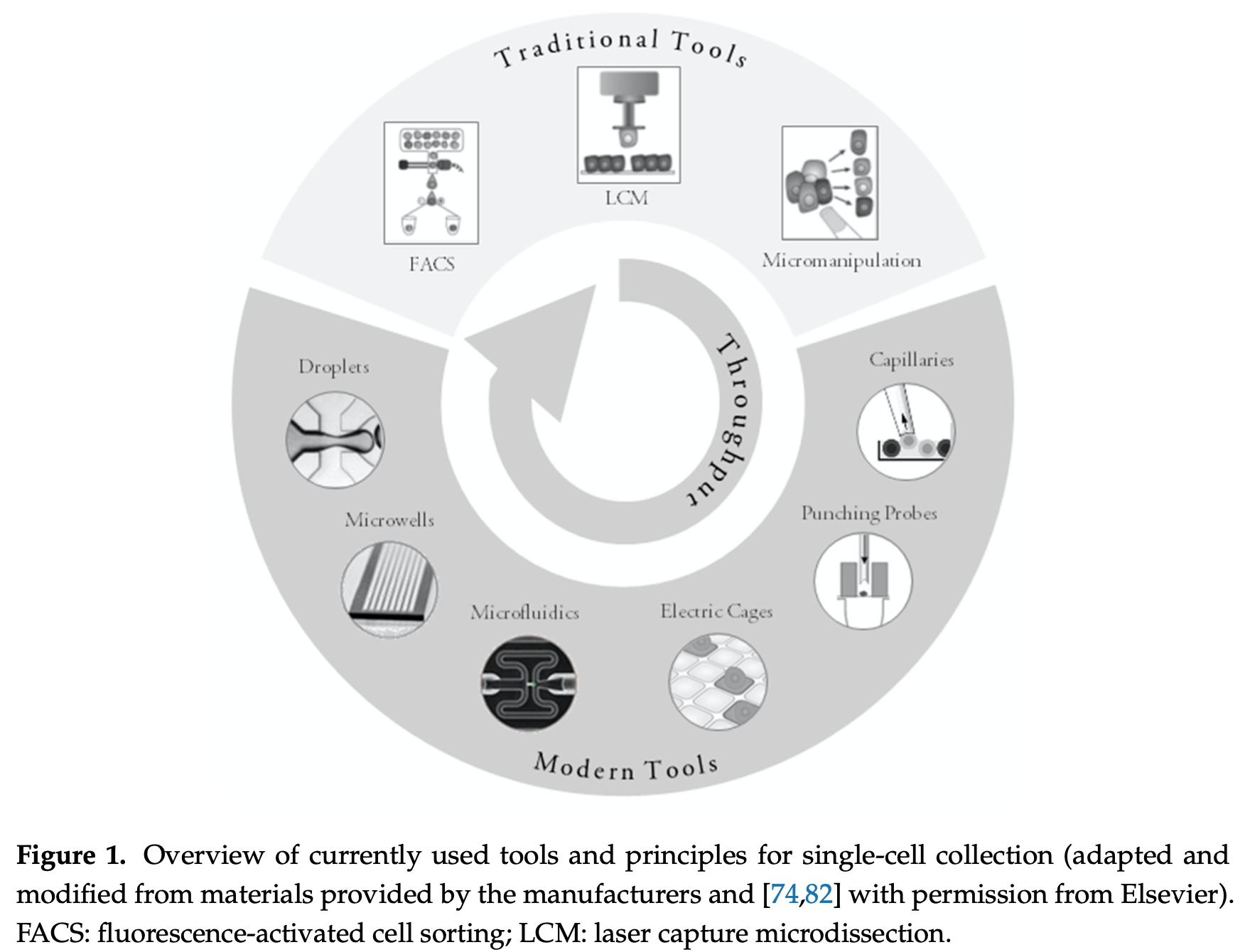
Cell Sorting Tools
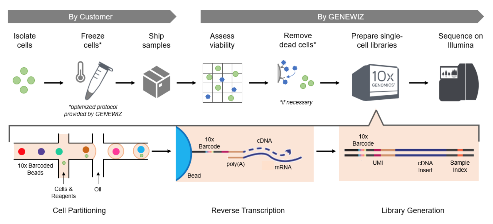
A common protocol comes from a company called 10x Genomics. Below is an overview of the cell sorting options available to researchers just to give you a quick impression of the variety of approaches.
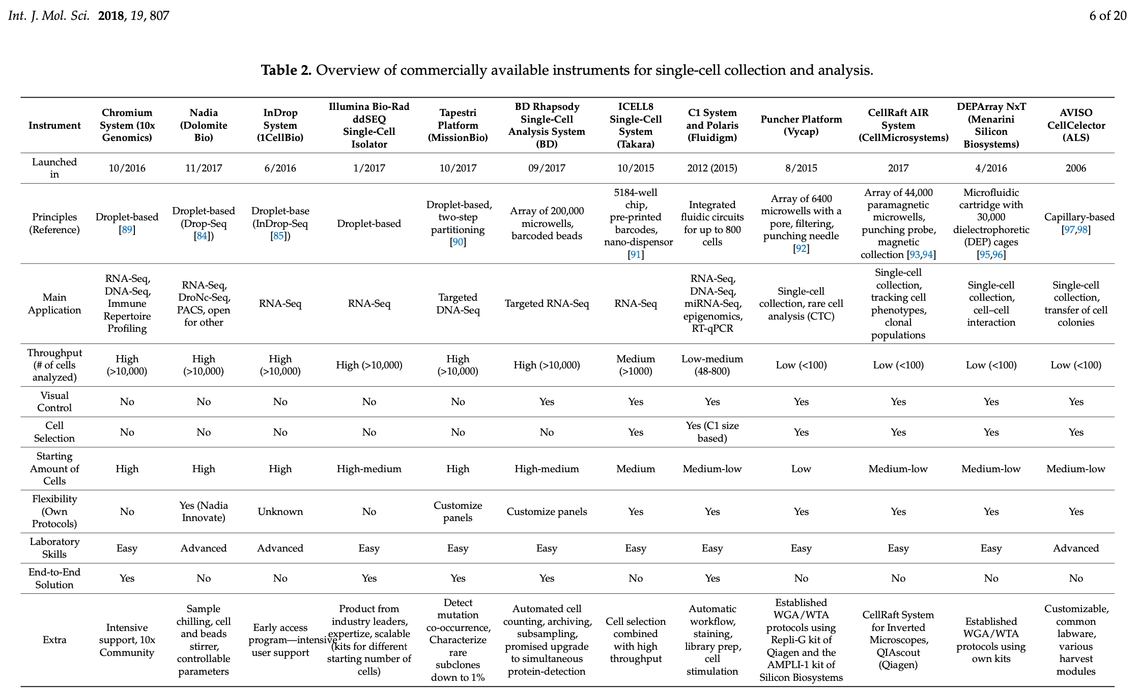
Cell Sorting Tools
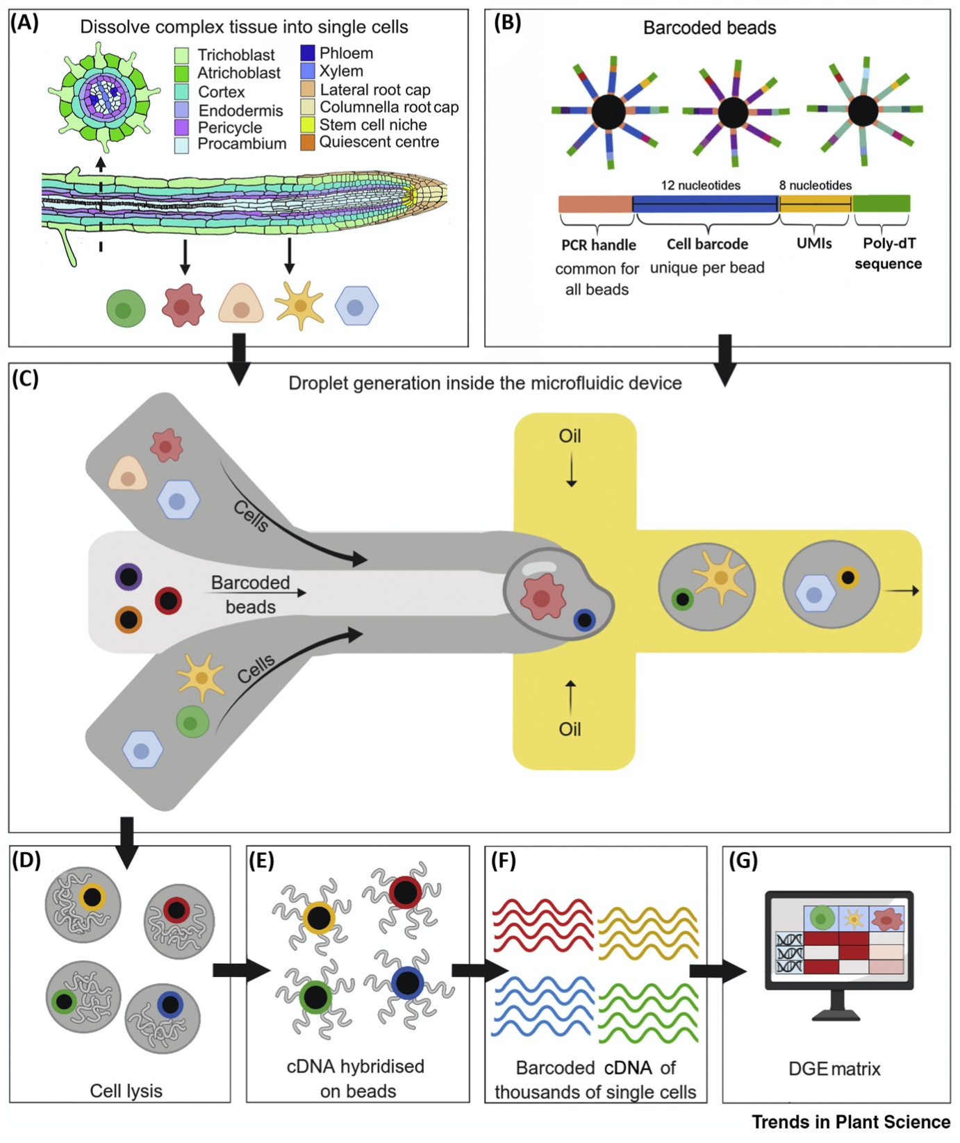
2.1.2 Once the single cells are isolated, how do we keep track of them? How do we know which cells belong to which sequences?
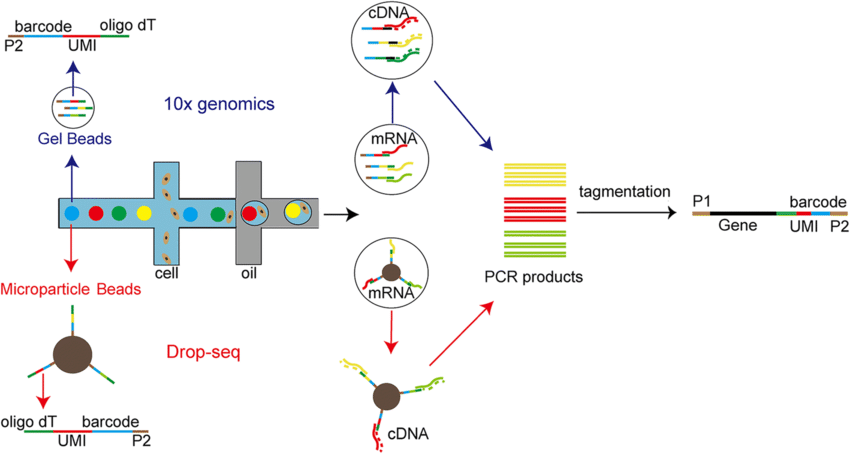
Droplets and UMIs
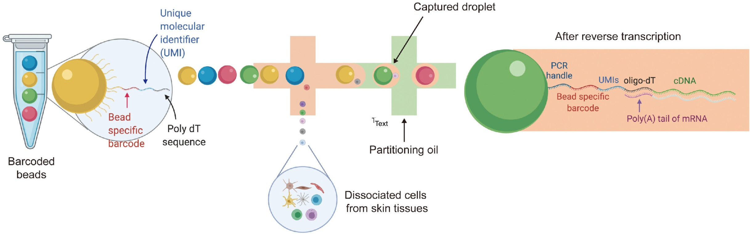
Cell Sorting Tools
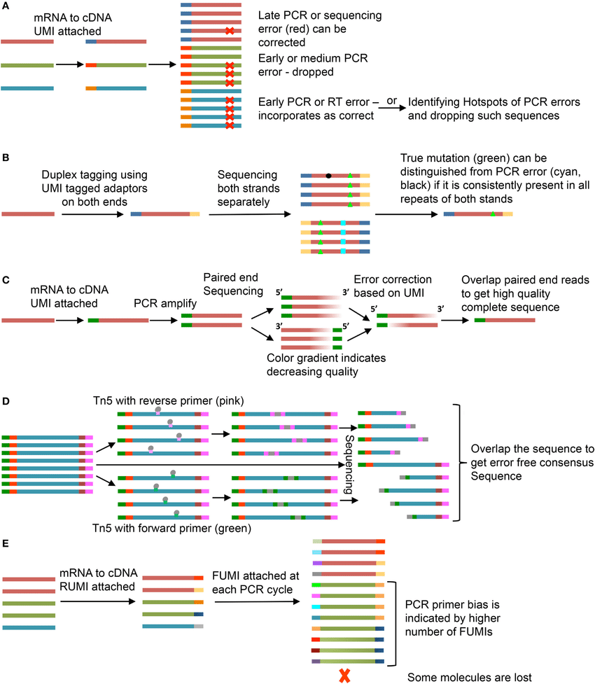
What does the UMI do?
UMIs are oligonucleotides consisting of random bases.
- Far more UMIs in the library than target DNA molecules so that ach target DNA molecule gets tagged with unique UMI
- Target DNA molecule + UMI gets carried forward to amplification
- Reads can later be grouped by UMI to generate a consensus sequence from all of the reads that contain one specific UMI
https://www.youtube.com/watch?v=gMzzXFMyM5g
UMIs
What does the Barcode do?
What does the Poly dT do?
2.2 Analysis Sequencing Data
Biological Context for interpreting scRNA-Seq Data and Data Analysis
This is an introduction to concepts. The purpose is to familiarize you with steps in an scRNA-Seq analysis workflow. Really, I hope that you understand what the purpose of the data processing steps are.
We are going to approach our learning using a journal-club model. I see that all of you are researchers and are likely very familiar with academic research publications and journal clubs. We will dissect a review paper from 2019 published in Molecular Systems Biology, titled “Current best practices in single cell RNA-seq analysis: a tutorial.”
This paper is paired with a tutorial freely available on github. These tutorials are not the same tutorials that we will cover in the course, providing an opportunity for extra practice as homework during the week of the workshop or afterward.
Luecken, M. D., & Theis, F. J. (2019). Current best practices in single‐cell RNA‐seq analysis: a tutorial. Molecular systems biology, 15(6), e8746.
https://www.github.com/theislab/single-cell-tutorial.
2.2.1 Objectives:
1.) scRNA-Seq Workflow:
- To be able to recognize, select, and design an scRNA-Seq workflow
2.) Pre Processing and Visualization:
3.) Quality Control:
To distinguish between cell count per depth, genes detected per cell, count depth distribution, mitochondrial read fractions.
To be able to interpret quality control metrics
4.) Normalization
5.) Data correction and integration
Regressing out biological effects
Regressing out technical effects
Batch effects and data integration
Expression recovery
6.) Feature selection, dimensionality reduction and visualization
Feature Selection
Dimensionality reduction
Visualization
7.) Stages of Pre-Processed data
Five stages of data processing
Three pre-processing layers
Downstream analysis
8.) Clustering analysis
Clustering
Cluster Annotation
Compositional Analysis
9.) Trajectory analysis
Trajectory interference
Gene expression dynamics
Metastable states
10.) Cell Level Analysis unification
11.) Gene-level analysis
Differential Expression testing
Gene set analysis
Gene regulatory networks
Keep an eye out for references to the following analysis tools, because you will be using them later on in the workshop:
Cell Ranger
Seurat
2.2.2 scRNA-Seq Workflow:
To be able to recognize, select, and design an scRNA-Seq workflow to answer your own question.
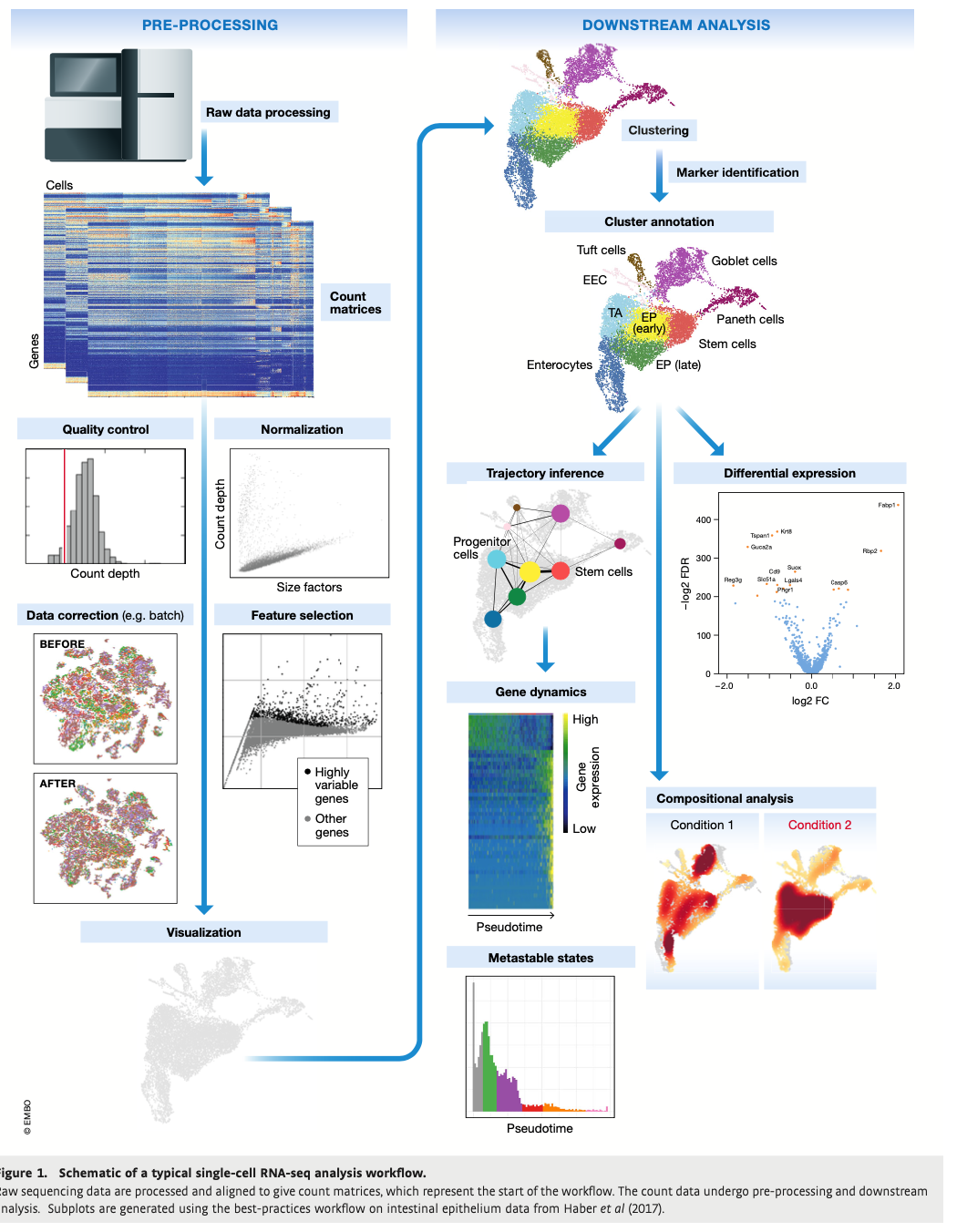
Analysis Workflow
Questions:
1.) To get from a cluster to an annotated cluster, what do we need match up to the to the cluster data? See Figure 1.
Answer: Marker Identifiers
2.) The barcode details listed below indicate that a cell has a broken membrane. Why?
Barcodes with a low count depth
few detected genes
high fraction of mitochondrial counts
Answer: After nuclear DNA leaks through a broken nuclear membrane, the only DNA left in a cell is the mitochondrial DNA.
Keep in mind that there are always other implications to consider. For example: Cells involved in respiration ALSO have a high mitochondrial count.
2.2.3 Processing and Visualization
1.) Raw Data
2.) Processed data
molecular counts (count matrices)
read counts (read matrices)
UMIs
Cell Ranger
Quality Control (QC)
Assigning reads to cellular barcodes (demultiplexing)
Assigning reads to mRNA molecules of origin (demultiplexing)
genome alignment
quantification
3.) Doublets
Mistake whereby a barcode may tag multiple cells instead of one
like 2 cells in a droplet
4.) Empty Droplet/Well
Mistake where no cells are tagged
0 cells in droplet
2.2.4 Quality Control:
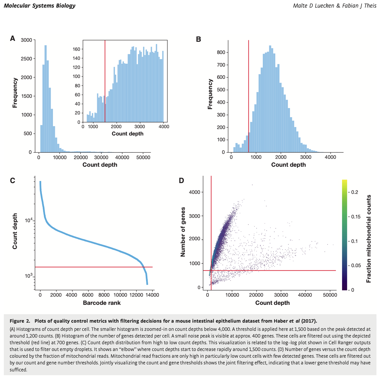
To distinguish between cell count per depth, genes detected per cell, count depth distribution, and mitochondrial read fractions. See Figure 2.
We will be regularly referring to “covariates” so it is important to keep in mind what a covariate is.
With respect to quality control in scRNA-seq, covariates are:
- counts per barcode (count depth)
- genes per barcode
- fractions of counts from mitochondrial genes
Run all QC Covariates (Cojointly) and cross reference the results of all three. Covariate dependence.
Questions:
What about barcodes that have
- unexpectedly high counts
- large number of detected genes?
What might that indicate?
- Answer: Could be doublets
- A doublet is where multiple cells are captured together
- in a microfluidic droplet
What might a quiescent cell population’s barcode details look like?
- Answer:
- low counts
- low genes
What might a QC Covariates show for cells that are larger in size?
- Answer:
- high cell counts
Should thresholds be set permissively?
- Answer: yes
- as permissively as possible
Why? - Don’t want to filter out viable cell populations.
What if you don’t filter?
- Only lowest count depth and lowest gene per barcode should be considered non-viable
Quality Control
2.2.5 Normalization
With normalization we are trying to get the correct relative gene expression abundances between cells. We are also trying to get uniform variance to satisfy assumptions of downstream tools.
There are many different methods ranging from:
Shifted logarithm
+ Adjusts for a size factor and adds a pseudocount before taking the logartihm
+ Simple and fast
Analytic Pearson residuals
+ Tries to adjust for technical variation while preserving biological variation
+ Takes into account the count depth
+ Normalized values can be positive or negative (lower counts than expected based on average expression of the gene and the sequencing depth of the cell)
2.2.6 Feature Selection
You can get expression values for up to 25,000 genes in a human singls-cell RNA-seq dataset.
Many genes won’t be informative for any given experimental inquiry. The goal is to obtain 500-2000 informative genes.
Single cell RNA approaches contain a lot of drop outs because of limited RNA. Genes with zero or very low counts are removed. Focus on genes that are highly variable across cells.
2.2.7 Dimension Reduction
2.2.7.1 Dimensionality reduction
Dimensionality reduction is done to:
- To ease downstream computational burden
- To reduce noise in the data
- To reduce redundancy in the data
- To visualize data
Popular dimensionality reduction techniques:
- Principal Component Analysis (PCA)
- Highly interpretable
- Linear approach to reduce dimensions
- Computationally efficient
- But scRNA-seq is sparse and non-linear
- Doesn’t reduce dimensions as much as non-linear methods
- tSNE (t-distributed stochastic neighbor embedding)
- Graph-based, non-linear approach
- Maintains local structure really well
- Computationally intensive
- UMAP (uniform manifold approximation and projection)
- Graph based, non-linear method
- Maintains local and global structure
- Relatively fast
2.2.8 Data correction and integration
2.2.8.1 Batch effects
These include technical variation introduced by differences in how samples are handled during collection or processing, differences in experimental protocols or even from differences in sequencing depths but the source of variation is often hard to pinpoint.
Batch effects can mask variation in rare cell populations and other important biological differences.
The recommendation is to be lenient on batch effect removal as you can remove important biological variation if you are too aggressive.
Basic steps in correcting for batch effects:
- Reduce dimensionality (improves signal to noise ratio)
- Model and remove the batch effect
- Project into high-dimensional space (opt)
Different types of batch correct are available:
Global models
- From bulk RNA-seq
- Assumes the batch effect is consistent across all cells
- Example: comBat
Linear embedding models
- Focuses on local neighborhoods of similar cells across batches
- This method is locally adaptive and non-linear
- Examples: Seurat and Harmony
Graph-based models
- Fast
- Connects cells from different batchs but prunes these connections to account for cell type differences
- Example: Batch-Balanced k-Nearest Neighbor (BBKNN)
Deep Learning models
- Usually based on autoencoder networks
- Can integrate cell identity labels to help maintain biological variation
- Examples: scVI, scANVI, and scGen

UMAP
2.2.8.2 Regressing out biological effects
Cell cycle markers, conserved
- Across tissue
- Across spieces
- Do you want to study effects of cell-cycle markers?
- Do you want to study something else?
How to regress out Cell-Cycle markers
- simple linear regression
- against a cell cycle score
Where does this score come from?
- Lists of marker genes in literature
- Macosko et al, 2015
Some argue that normalizing for Cell Size already accounts for Cell-Cycle effects
- McDavid et al, 2016
- https://www.nature.com/articles/srep33892
Other markers: Ribosome Mitochondrial